
Self-Labeled Techniques for Semi-Supervised Learning: Taxonomy, Software and Empirical Study
This Website contains complementary material to the paper:
I. Triguero, S. García, and F. Herrera, Self-Labeled Techniques for Semi-Supervised Learning: Taxonomy, Software and Empirical Study.
Summary:
- Abstract
- Experimental Framework
- Results obtained
- Statistical Tests
- A Semi-Supervised Learning Module for KEEL
I. Triguero, S. García, and F.Herrera, Self-Labeled Techniques for Semi-Supervised Learning: Taxonomy, Software and Empirical Study.
Abstract
Semi-supervised classification methods tackle training sets with large amounts of unlabeled data and a small quantity of labeled data. Among other approaches, self-labeled techniques iteratively enlarge the labeled dataset accepting that their own predictions are correct. In this article we provide a survey of self-labeled methods, proposing a taxonomy and analyzing empirically their performance with a large number of datasets. Note is then taken of which models are the most promising and/or unexplored alternatives for practitioners of this growing field. Moreover, a semi-supervised learning software package has been developed, integrating analyzed methods and datasets.
Experimental framework
Semi-Supervised Classification Data sets
The experimentation is based on 55 standard classification datasets taken from the UCI repository UCI Machine Learning Repository and the KEEL-dataset repository. Following table summarizes the properties of the selected data sets. It shows, for each data set, the number of examples (#Ex.), the number of attributes (#Atts.), and the number of classes (#Cl.).
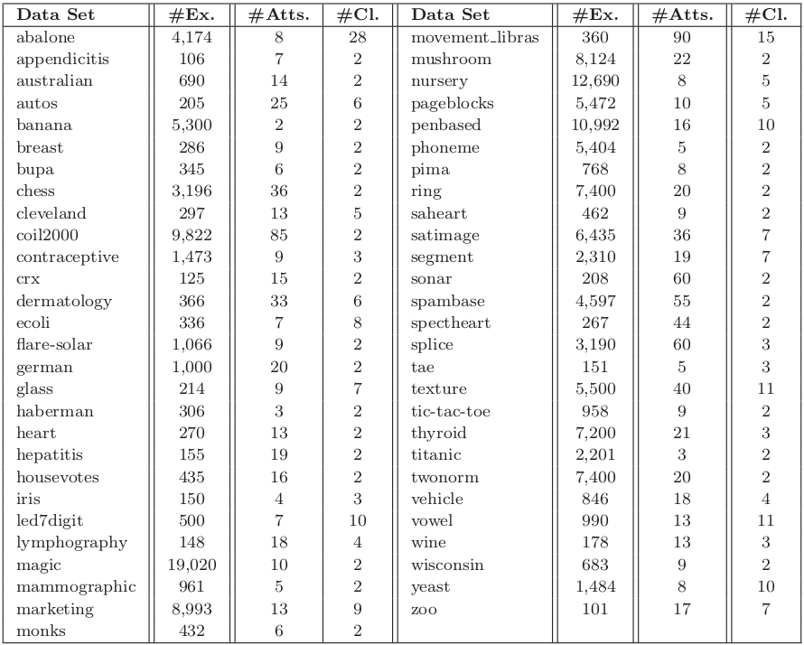
Table 1. Summary description for classification data sets
These data sets have been partitioned using the ten fold cross-validation procedure, that is, the data set has been split into 10 folds, each one contains the 10\% of the examples of the data set. For each generated fold, a given algorithm is trained with the examples contained in the rest of folds (training partition) and then tested with the current fold. It is noteworthy that test partitions are kept aside to evaluate the performance of the learned hypothesis.
In order to study the influence of the amount of labeled data, we take four different ratios when dividing the training set: 10%, 20%, 30% and 40%. Therefore, this experimental study involves a total of 220 data sets.
You can also download all these datasets here:
- Semi-Supervised Classification Data sets (10% labeled rate)

- Semi-Supervised Classification Data sets (20% labeled rate)
- Semi-Supervised Classification Data sets (30% labeled rate)
- Semi-Supervised Classification Data sets (40% labeled rate)
Furthermore, we will use 9 high dimensional benchmarks data sets extracted from:
http://olivier.chapelle.cc/ssl-book/benchmarks.html These problems have been also partitioned using a ten fold-cross validation scheme in order to evaluate them in terms of transductive and inductive capabilities. Each training partition is divided into labeled and unlabeled examples. We ensure that each partition contains at least one point of each class. Apart from this, there is no bias in the labeling process. We will use two splits: 10 labeled points and 100 labeled point (the remaining data is considered as unlabeled). The following table describes the main characteristics of these problems.
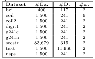
Table 2. Summary description for high dimensional data sets
- High dimensional data sets (10 labeled examples)
- High dimensional data sets (100 labeled examples)
Parameters and base classifiers
The selected configuration parameters are common for all problems, and hey were selected according to the recommendation of the corresponding authors of each algorithm. The approaches analyzed should be as general and flexible as possible. A good choice of parameters assists them to perform better over different data sources, but their operations should allow to obtain good enough results although the parameters are not optimized for a specific data set. This is the main purpose of this experimental survey, to show the generalization in performance of each self-labeled technique. The configuration parameters of all the methods are specified in Table 2.
Some of the self-labeled methods have been designed with one or more specific base classifier/s. In this study, these algorithms maintain their used classifier/s, however, the interchange of the base classifier is allowed in other approaches. Specifically, they are: SelfTraining, Co-Training, TriTraining, DE-TriTraining, Rasco and Rel-Rasco. In this study, we select four classic and well-known classifiers in order to find differences in performance among these self-labeled methods. They are K-Nearest Neighbor, C4.5, Naive Bayes and SVM and their respective configuratio parameters are shown in Table 3. A brief description of the base classifiers and their associated confidence predictions computation are enumerated next:
- K-Nearest Neighbor (KNN): This is one of the simplest and effective method based on dissimilarities among a set of instances. It belong to the lazy learning family of methods which do not build a model during the learning process. With this method, confidence predictions can be approximated by the distance to the currently labeled set.
- C4.5: This is a well-known decision tree algorithm. It induces classification rules in the form of decision trees for a given training set. The decision tree is built with a top-down scheme, using the normalized information gain (difference in entropy) that is obtained from choosing an attribute for splitting the data. The attribute with the highest normalized information gain is the one used to make the decision. Confidence predictions are obtained from the accuracy of the leaf that makes the prediction. The accuracy of a leaf is the percentage of correctly classified train examples from the total number of covered train instances.
- Naive Bayes (NB): Its aim is to construct a rule which will allow us to assign future objects to a class, assuming independence of attributes when probabilities are established. For continuous data, we follow a typical assumption in which continuous values associated with each class are distributed according to a Gaussian distribution. The probabilities' extraction is straightforward, due to the fact that this method explicitly computes the probability belonging to each class for the given test instance.
- Support Vector Machines (SVM): It maps the original input space into a higher dimensional feature space using a certain kernel function. In the new feature space, the SVM algorithm searches the optimal separating hyperplane with maximal margin in order to minimize an upper bound of the expected risk instead of the empirical risk. Specifically, we use SMO training algorithm to obtain the SVM base classifiers. Using a logistic model, we can use the probabilities estimate from the SMO as the confidence for the predicted class.
Table 2: Parameter specification for the self-labeled used in the experimentation
| Method | Parameters |
|---|---|
| Self-Training | MAX_ITER = 40 |
| Co-Training | MAX_ITER = 40, Initial Unlabeled Pool=75 |
| Democratic-Co | Classifiers = 3NN, C4.5, NB |
| SETRED | MAX_ITER = 40, Threshold = 0.1 |
| TriTraining | No parameters specified |
| DE-TriTraining | Number of Neighbors k = 3, Minimum number of neighbors = 2 |
| CoForest | Number of RandomForest Classifiers = 6, Threshold = 0.75 |
| Rasco | MAX_ITER = 40, Number of Views/Classifiers = 30 |
| Co-Bagging | MAX_ITER = 40, Committee members = 3, Ensemble Learning = Bagging, Pool U = 100 |
| Rel-Rasco | MAX_ITER = 40, Number of Views/Classifiers = 30 |
| CLCC | Number of RandomForest Classifiers = 6, Threshold = 0.75, Manipulative beta parameter = 0.4, Initial number of cluster = 4, Running Frequency z = 10, best center sets = 6, Optional Step = True |
| APSSC | Spread of the Gaussian = 0.3, Evaporation Coefficient = 0.7, MT = 0.7 |
| SNNRCE | Threshold = 0.5 |
| ADE-CoForest | Number of RandomForest Classifiers = 6, Threshold = 0.75, Number of Neighbors k = 3, Minimum number of neighbors = 2 |
Table 3: Parameter specification for the base classifiers employed in the experimentation
| Method | Parameters |
|---|---|
| KNN | K = 3, Euclidean distance |
| C4.5 | pruned tree, confidence = 0.25, 2 examples per leaf |
| NB | No parameters specified |
| SMO | C = 1.0, Tolerance Parameter = 0.001, Epsilon= 1.0E-12, Kernel Type = Polynomial, Polynomial degree = 1, Fit logistic models = true |
Results obtained
In this section, we report the full results obtained in the experimental study. We present these data in xls and ods files available for download. These files are composed by 5 sheets: Transductive Accuracy results, Transductive Kappa results, Inductive Accuracy results, Inductive Kappa results and Summary of results.
Each sheet is organized as follows: each data set is put in the rows of the file and each self-labeled method performance results are placed in the columns of the file. There are two columns for every method: one representing the average performance results (accuracy or kappa rates) and another with the standard deviation for that average performance results. Additionally, in the summary sheet the algorithms are ordered from the best to the worst accuracy/kappa obtained in both transductive and inductive results and includes the analysis of the behavior in binary and multi-class data sets.
Table 4: Results obtained
| Labeled Ratio | xls file | ods file |
| 10% | ||
| 20% | ||
| 30% | ||
| 40% |
Furthermore, the comparative study between oustanding models and the supervised learning paradigm is included in the following file:
Table 5: How far is semi-supervised learning from the traditional supervised learning paradigm?
| File | xls file | ods file |
| Semi-Supervised Learning Vs Supervised Learning |
Statistical tests
Statistical analysis are carried out by means of nonparametric statistical tests. The reader can look up the Statistical Inference in Computational Intelligence and Data Mining web page for details in nonparametric statistical analysis.
The Wilcoxon test is used in order to conduct pairwise comparisons among all discretizers considered in the study. Specifically, the Wilcoxon test is adopted in this study considering a level of significance equal to α = 0.1.
In Table 5 we provide the results of the Wilcoxon test for every performance measure used in this study. For each comparison we provide two different files: a pdf file with the detailed results of the Wilcoxon test and a second file with the summary associated to it.
Table 6: Wilcoxon Test results for each performance measure used in the study
| Labeled Ratio | Phase | Detailed Wilcoxon test | Summary of the Wilcoxon test |
|---|---|---|---|
| 10% | Transductive | ||
| Inductive | |||
| 20% | Transductive | ||
| Inductive | |||
| 30% | Transductive | ||
| Inductive | |||
| 40% | Transductive | ||
| Inductive |
Table 7 summarizes all possible comparisons involved in the Wilcoxon test among all the methods considered, considering accuracy/kappa results. In these files, tables present, for each method in the rows, the number of self-labeled methods outperformed by using the Wilcoxon test under the column represented by the '+' symbol. The column with the '+-' symbol indicates the number of wins and ties obtained by the method in the row.
Table 7: Wilcoxon Test summary results
| Phase | Measure | pdf file |
|---|---|---|
| Transductive | Accuracy | |
| Kappa | ||
| Inductive | Accuracy | |
| Kappa |
Furthermore, we will use the Friedman test, in the global analysis, to analyze differences between the methods stressed as outstanding with a multiple comparison analysis. The Bergmann-Hommel procedure is applied as a post-hoc procedure to find out which algorithms are distinctive in n*n comparisons.
Table 8: Multiple Comparison test between outstanding methods.
| Phase | Measure | xls file | ods file |
|---|---|---|---|
| Transductive | Accuracy | ||
| Kappa | |||
| Inductive | Accuracy | ||
| Kappa |
A Semi-Supervised Learning Module for KEEL
As consequence of this work, we have developed a complete SSL framework which have been integrated into the KEEL (Knowledge Extraction based on Evolutionary Learning) tool http://sci2s.ugr.es/keel/.
You can download the KEEL Sofware Tool here. Since the KEEL Sofware Tool is an open source (GPLv3) tool, its source code it is also available for its usage here.
![]()
![]()
The source code of the SSL module can be downloaded from here.
It is written in the Java programming language. Although it is developed to be run inside the KEEL environment, it can be also executed on a standard Java Virtual Machine. To do this, it is only needed to place the training datasets at the same folder, and write a script which contains al the relevant parameters of the algorithms (see the KEEL reference manual, section 3; located under the KEEL Software Tool item of the main menu).
The KEEL version with the SSL module can be downloaded from here.
Esentially, to generate a experiment with this modified version of KEEL, it is needed to perform the following steps:
- Execute the KEEL GUI with the command: java -jar GraphInterKeel.jar.
- Select Modules, and then Semi-Supervised Learning.
- Select the data sets desired to use, and click on the main window to place them.
- Click on the second icon of the left bar, select the SSL method desired, and click on the main window to place it.
- Click on the last icon of the left bar, and create some arcs which joins all the nodes of the experiments.
- Click on the Run Experiment icon, located at the top bar.
This way, it is possible to generate an experiment ready to be executed on any machine with a Java Virtual Machine installed.