
Noisy Data in Data Mining
This web is organized according to the following summary:![]()
- Introduction to noise in data mining
- Noise types: class (label) noise and attribute noise
- Evaluating the classifier behavior with noisy data: metrics BRM, RLA and ELA
- Using noise filters to reduce noise's effects
- SCI2S related approaches
- SMOTE-IPF: Dealing with noisy data in imbalanced domains
- INFFC: An iterative filter based on the fusion of classifiers with noise sensitivity control
- Noise filtering efficacy prediction by data complexity measures
- Quantifying the benefits of using MCS with noise
- Advantages of OVO scheme in the presence of noise
- Using the One-vs-One decomposition to improve the performance of class noise filters
- Datasets used
- Noise Data Software
- Noisy data bibliography
This Website contains a short introduction to Noisy Data together with the more relevant bibliography and it also contains the complementary material to the SCI2S research group papers on Noisy Data in Data Mining.
Introduction to noise in data mining
Real-world data, which is the input of the Data Mining algorithms, are affected by several components; among them, the presence of noise is a key factor (R.Y. Wang, V.C. Storey, C.P. Firth, A Framework for Analysis of Data Quality Research, IEEE Transactions on Knowledge and Data Engineering 7 (1995) 623-640 doi: 10.1109/69.404034). Noise is an unavoidable problem, which affects the data collection and data preparation processes in Data Mining applications, where errors commonly occur. Noise has two main sources (X. Zhu, X. Wu, Class Noise vs. Attribute Noise: A Quantitative Study, Artificial Intelligence Review 22 (2004) 177-210 doi: 10.1007/s10462-004-0751-8): implicit errors introduced by measurement tools, such as different types of sensors; and random errors introduced by batch processes or experts when the data are gathered, such as in a document digitalization process.
The performance, which we usually want to maximize, of the classifiers built under such circumstances will heavily depend on the quality of the training data, but also on the robustness against noise of the classifier itself (as it is represented in the following scheme).
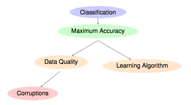
Hence, classification problems containing noise are complex problems and accurate solutions are often difficult to achieve. The presence of noise in the data may affect the intrinsic characteristics of a classification problem, since these corruptions could introduce new properties in the problem domain. For example, noise can lead to the creation of small clusters of examples of a particular class in areas of the domain corresponding to another class, or it can cause the disappearance of examples located in key areas within a specific class. The boundaries of the classes and the overlapping between them are also factors that can be affected as a consequence of noise. All these alterations difficult the knowledge extraction from the data and spoil the models obtained using that noisy data when they are compared to the models learned from clean data, which represent the real implicit knowledge of the problem. Therefore, data gathered from real-world problems are never perfect and often suffer from corruptions that may hinder the performance of the system in terms of (X. Wu, X. Zhu, Mining with noise knowledge: Error-aware data mining, IEEE Transactions on Systems, Man, and Cybernetics 38 (2008) 917-932 doi: 10.1109/TSMCA.2008.923034):
- the classification accuracy;
- building time;
- size and interpretability of the classifier.
On the other hand an excellent review on class (label) noise can be found in Frenay, B.; Verleysen, M., "Classification in the Presence of Label Noise: A Survey," in Neural Networks and Learning Systems, IEEE Transactions on , vol.25, no.5, pp.845-869, May 2014
doi: 10.1109/TNNLS.2013.2292894.
Noise types: class (label) noise and attribute noise
1. Simulating the noise of real-world datasets
2. Creating a noisy dataset from the original one
A large number of components determine the quality of a dataset (R.Y. Wang, V.C. Storey, C.P. Firth, A Framework for Analysis of Data Quality Research, IEEE Transactions on Knowledge and Data Engineering 7 (1995) 623-640 doi: 10.1109/69.404034). Among them, the class labels and the attribute values directly influence the quality of a classification dataset. The quality of the class labels refers to whether the class of each example is correctly assigned; otherwise, the quality of the attributes refers to their capability of properly characterizing the examples for classification purposes - obviously, if noise affects attribute values, this capability of characterization and therefore, the quality of the attributes, is reduced. Based on these two information sources, two types of noise can be distinguished in a given dataset (see the following figure) (X. Zhu, X. Wu, Class Noise vs. Attribute Noise: A Quantitative Study, Artificial Intelligence Review 22 (2004) 177-210 doi: 10.1007/s10462-004-0751-8):
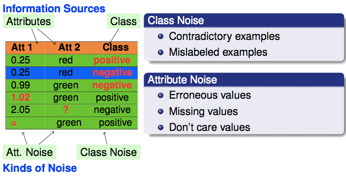
1. Class noise (label noise). This occurs when an example is incorrectly labeled. Class noise can be attributed to several causes, such as subjectivity during the labeling process, data entry errors, or inadequacy of the information used to label each example. Two types of class noise can be distinguished:
- Contradictory examples (M.A. Hernández, S.J. Stolfo, Real-world Data is Dirty: Data Cleansing and The Merge/Purge Problem, Data Mining and Knowledge Discovery 2 (1998) 9-37 doi: 10.1023/A:1009761603038): duplicate examples have different class labels. In the figure placed above the two examples (0.25, red, class = positive) and (0.25, red, class = negative) are contradictory examples, since they have the same attribute values and a different class.
- Misclassifications (X. Zhu, X. Wu, Q. Chen, Eliminating class noise in large datasets, in: Proceeding of the Twentieth International Conference on Machine Learning, pp. 920-927): examples that are labeled as a class different from the real one. In the figure placed above the example (0.99, greee, class = negative) is a mislabeled example, since its class label is wrong, and it would be "positive".
There exist a profuse literature in class noise, also called label noise, as in the recent and extensive review on this type of noise Frenay, B.; Verleysen, M., "Classification in the Presence of Label Noise: A Survey," in Neural Networks and Learning Systems, IEEE Transactions on , vol.25, no.5, pp.845-869, May 2014 doi: 10.1109/TNNLS.2013.2292894.
2. Attribute noise. This refers to corruptions in the values of one or more attributes. Examples of attribute noise are:
- Erroneous attribute values. In the figure placed above, the example (1.02, green, class = positive) has its first attribute with noise, since it has wrong value.
- Missing or unknown attribute values. In the figure placed above, the example (2.05, ?, class = negative) has attribute noise, since we do not know the value of the second attribute.
- Incomplete attributes or "do not care" values. In the figure placed above, the example (=, green, class = positive) has attribute noise, since the value of the first attribute do not affect the rest of values of the example, including the class of the example.
Considering class and attribute noise as corruptions of the class labels and attribute values, respectively, is common in real-world data. Because of this, these types of noise haven been also considered in many works in the literature. For instance, in (X. Zhu, X. Wu, Class Noise vs. Attribute Noise: A Quantitative Study, Artificial Intelligence Review 22 (2004) 177-210 doi: 10.1007/s10462-004-0751-8), the authors reached a series of interesting conclusions, showing that attribute noise is more harmful than class noise or that eliminating or correcting examples in datasets with class and attribute noise, respectively, may improve classifier performance. They also showed that attribute noise is more harmful in those attributes highly correlated with the class labels. In (D. Nettleton, A. Orriols-Puig, A. Fornells, A Study of the Effect of Different Types of Noise on the Precision of Supervised Learning Techniques, Artificial Intelligence Review 33 (2010) 275-306 doi: 10.1007/s10462-010-9156-z), the authors checked the robustness of methods from different paradigms, such as probabilistic classifiers, decision trees, instance based learners or support vector machines, studying the possible causes of their behaviors.
However, most of the works found in the literature are only focused on class noise. In (Bootkrajang, J., Kabán, A. : Multi-class classification in the presence of labelling errors. In: European Symposium on Artificial Neural Networks 2011 (ESANN 2011), pp. 345-350 (2011)), the problem of multi-class classification in the presence of labeling errors was studied. The authors proposed a generative multi-class classifier to learn with labeling errors, which extends the multi-class quadratic normal discriminant analysis by a model of the mislabeling process. They demonstrated the benefits of this approach in terms of parameter recovery as well as improved classification performance. In (Hernández-Lobato, D., Hernández-Lobato, J.M., Dupont, P. : Robust multi-class gaus- sian process classification. In: Anual Conference on Neural Information Processing Systems (NIPS 2011), pp. 280-288 (2011)), the problems caused by labeling errors occurring far from the decision boundaries in Multi-class Gaussian Process Classifiers were studied. The authors proposed a Robust Multi-class Gaussian Process Classifier, introducing binary latent variables that indicate when an example is mislabeled. Similarly, the effect of mislabeled samples appearing in gene expression profiles was studied in (Zhang, C., Wu, C., Blanzieri, E., Zhou, Y., Wang, Y., Du, W., Liang, Y. : Methods for labeling error detection in microarrays based on the effect of data perturbation on the regression model. Bioinformatics 25(20), 2708-2714 (2009) doi: 0.1093/bioinformatics/btp478). A detection method for these samples was proposed, which take advantage of the measuring effect of data perturbations based on the support vector machine regression model. They also proposed three algorithms based on this index to detect mislabeled samples. An important common characteristic of these works, also considered in this paper, is that the suitability of the proposals was evaluated on both real-world and synthetic or noisy-modified real-world datasets, where the noise can be somehow quantified.
Simulating the noise of real-world datasets
Checking the effect of noisy data on the performance of classifier learning algorithms is necessary to improve their reliability and has motivated the study of how to generate and introduce noise into the data. Noise generation can be characterized by three main characteristics:
- The place where the noise is introduced. Noise may affect the input attributes or the output class, impairing the learning process and the resulting model.
- The noise distribution. The way in which the noise is present can be, for example, uniform or Gaussian.
- The magnitude of generated noise values. The extent to which the noise affects the dataset can be relative to each data value of each attribute, or relative to the minimum, maximum and standard deviation for each attribute.
In real-world datasets the initial amount and type of noise present are unknown. Therefore, no assumptions about the base noise type and level can be made. For this reason, these datasets are considered to be noise free, in the sense that no recognizable noise has been induced into them. In order to control the amount of noise in each dataset and check how it affects the classifiers, noise is introduced into each dataset in a supervised manner in the literature. The two types of noise considered, class and attribute noise, have been modeled using four different noise schemes in the literature; in such a way, the presence of a noise level x% of those types of noise will allow one to simulate the behavior of the classifiers in these scenarios:
- Class noise usually occurs on the boundaries of the classes, where the examples may have similar characteristics - although it can occur in any other area of the domain. Class noise is introduced in the literature using an uniform class noise scheme (randomly corrupting the class labels of the examples) and a pairwise class noise scheme (labeling examples of the majority class with the second majority class). Considering these two schemes, noise affecting any pair of classes and only the two majority classes are simulated, respectively.
- Uniform class noise. x% of the examples are corrupted. The class labels of these examples are randomly replaced by another one from the other classes.
- Pairwise class noise. Let X be the majority class and Y the second majority class, an example with the label X has a probability of x/100 of being incorrectly labeled as Y.
- Attribute noise can proceed from several sources, such as transmission constraints, faults in sensor devices, irregularities in sampling and transcription errors. The erroneous attribute values can be totally unpredictable, i.e., random, or imply a low variation with respect to the correct value. We use the uniform attribute noise scheme and the Gaussian attribute noise scheme in order to simulate each one of the possibilities, respectively. We introduce attribute noise in accordance with the hypothesis that interactions between attributes are weak; as a consequence, the noise introduced into each attribute has a low correlation with the noise introduced into the rest.
- Uniform attribute noise. x% of the values of each attribute in the dataset are corrupted. To corrupt each attribute Ai, x% of the examples in the data set are chosen, and their Ai value is assigned a random value from the domain Di of the attribute Ai. An uniform distribution is used either for numerical or nominal attributes.
- Gaussian attribute noise. This scheme is similar to the uniform attribute noise, but in this case, the Ai values are corrupted, adding a random value to them following a Gaussian distribution of mean = 0 and standard deviation = (max-min)/5, being max and min the limits of the attribute domain. Nominal attributes are treated as in the case of the uniform attribute noise.
Creating a noisy dataset from the original one
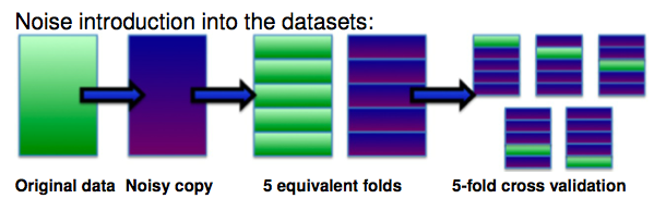
In order to create a noisy dataset from the original one, we must consider several facts, such as the type of noise, the place where the noise will be introduced or the number of folds of the cross validation (that is usually used to validate the classifiers built). The general scheme that must be performed is the following:
- A level of noise x%, of either class noise (uniform or pairwise) or attribute noise (uniform or Gaussian), is introduced into a copy of the full original dataset.
- Both datasets, the original one and the noisy copy, are partitioned into N equivalent folds, that is, with the same examples in each one.
- The training partitions are usually built from the noisy copy, whereas the test partitions are formed from examples from the base dataset (that is, the noise free dataset) in the case of class noise, whereas in the case of attribute noise, test partitions can be formed with the noisy copy or the base datasets, depending on what we want to study.
The following figure shows an example on how to introduce class noise using a 5-fold cross validation (the green folds are the test partitions, whereas the blue folds are the training partitions):
Evaluating the classifier behavior with noisy data: metrics BRM, RLA and ELA
Noise hinders the knowledge extraction from the data and spoils the models obtained using these noisy data when they are compared to the models learned from clean data from the same problem. In this sense, robustness is the capability of an algorithm to build models that are insensitive to data corruptions and suffer less from the impact of noise; that is, the more robust an algorithm is, the more similar the models built from clean and noisy data are. Thus, a classification algorithm is said to be more robust than another if the former builds classifiers which are less influenced by noise than the latter. Robustness is considered very important when dealing with noisy data, because it allows one to expect a priori the amount of variation of the learning method's performance against noise with respect to the noiseless performance in those cases where the characteristics of noise are unknown. It is important to note that a higher robustness of a classifier does not imply a good behavior of that classifier with noisy data, since a good behavior implies a high robustness but also a high performance without noise.
In the literature, the measures that are used to analyze the degree of robustness of the classifiers in the presence of noise compare the performance of the classifiers learned with the original (without controlled noise) data set with the performance of the classifiers learned using a noisy version of that data set. Therefore, those classifiers learned from noisy data sets that are more similar (in terms of results) to the noise-free classifiers will be the most robust ones. The robustness-based measures found in the literature are:
- The BRM metric [Y. Kharin, E. Zhuk, Robustness in statistical pattern recognition under contaminations of training samples., in: Proceedings of the 12th IAPR International Conference on Pattern Recognition, Vol. 2 - Conference B: Computer Vision and Image Processing (1994) 504-506 doi: 10.1109/ICPR.1994.576996]. This measure considers the performance of Bayesian Decision rule as a reference, which is considered as the classifier providing the minimal risk when the training data are not corrupted. Concretely, the next expression is used:
$$BRM_{x\%} = \frac{E_{x\%}-E}{E}$$
where $E_{x\%}$ is the risk (that we will understand as the classification error rate in our case) of the classifier at a noise level $x\%$ and $E$ is the risk of the Bayesian Decision rule without noise. This classifier is a theoretical decision rule, that is, it is not learned from the data, which depends on the data generating process. Its error rate is by definition the minimum expected error that can be achieved by any decision rule.
- The Relative Loss of Accuracy (RLA) [J.A. Sáez, J. Luengo, F. Herrera, Fuzzy rule based classification systems versus crisp robust learners trained in presence of class noise's effects: a case of study, in: 11th International Conference on Intelligent Systems Design and Applications (2011) 1229-1234 doi: 10.1109/ISDA.2011.6121827] . This metric is defined as:
$$RLA_{x\%} = \frac{A_{0\%}-A_{x\%}}{A_{0\%}}$$
where $A_{0\%}$ is the accuracy of the classifier with a noise level 0\%, and $A_{x\%}$ is the accuracy of the classifier with a noise level $x\%$. RLA evaluates the robustness as the loss of accuracy with respect to the case without noise $A_{0\%}$, weighted by this value $A_{0\%}$. This measure has two clear advantages: (i) it is simple and interpretable and (ii) to the same values of loss $A_{0\%}-A_{x\%}$, the methods having a higher value of accuracy without noise $A_{0\%}$ will have a lower RLA value.
- The Equalized Loss of Accuracy (ELA) [J.A. Sáez, J. Luengo, F. Herrera, Evaluating the classifier behavior with noisy data considering performance and robustness: The Equalized Loss of Accuracy measure. Neurocomputing, in press (2015), doi: 10.1016/j.neucom.2014.11.086]. This metric es defined as:
$$ELA_{x\%} = \frac{100-A_{x\%}}{A_{0\%}}$$
This measure used to evaluate the behavior of a classifier with noisy data overcomes some problems of the RLA measure: (i) it takes into account the noiseless performance $A_{0\%}$ when considering which classifier is more appropriate with noisy data. This fact makes ELA more suitable to compare the behavior against noise between 2 different classifiers. We must take into account that a benchmark data set might contain implicit and not controlled noise with a noise level $x = 0\%$, (ii) a classifier with a low base accuracy $A_{0\%}$ that is not deteriorated at higher noise levels $A_{x\%}$ is not better than another better classifier suffering from a low loss of accuracy when the noise level is increased.
Using noise filters to reduce noise's effects
Given the loss of accuracy produced by noise, the need of techniques to deal with it has been proved in previous works (X. Zhu, X. Wu, Class Noise vs. Attribute Noise: A Quantitative Study, Artificial Intelligence Review 22 (2004) 177-210). In the specialized literature, two ways have been proposed in order to mitigate the effects produced by noise:
- Adaptation of the algorithms to properly handle the noise (J.R. Quinlan, C4.5: programs for machine learning, Morgan Kaufmann Publishers, San Francisco, CA, USA, 1993 doi: 10.1007/BF00993309 , W.W. Cohen, Fast effective rule induction, in: Proceedings of the Twelfth International Conference on Machine Learning, Morgan Kaufmann Publishers, 1995, pp. 115-123). These methods are known as robust learners and they are characterized by being less influenced by noisy data.
- Preprocessing of the datasets aiming to remove or correct the noisy examples (Brodley, C.E., Friedl, M.A.: Identifying Mislabeled Training Data. Journal of Artificial Intelligence Research 11, 131-167 (1999) doi:10.1613/jair.606; Gamberger, D., Boskovic, R., Lavrac, N., Groselj, C.: Experiments With Noise Filtering in a Medical Domain. In: Proceedings of the Sixteenth International Conference on Machine Learning, pp. 143-151. Morgan Kaufmann Publishers (1999)).
However, even though both techniques can provide good results, drawbacks exist. The former depends on the classification algorithm - and therefore, the same result is not directly extensible to other learning algorithms, since the benefit comes from the adaptation itself. Moreover, this approach requires to change an existing method, which neither is always possible nor easy to develop. However, the latter requires the usage of a previous preprocessing step, which is usually time consuming. Furthermore, these methods are only designed to detect an specific type of noise and hence, the resulting data might not be perfect (X. Wu, X. Zhu, Mining with noise knowledge: Error-aware data mining, IEEE Transactions on Systems, Man, and Cybernetics 38 (2008) 917-932 doi: 10.1109/TSMCA.2008.923034). For these reasons, it is important to investigate other mechanisms, which could lead to decrease the effects caused by noise without neither needing to adapt each specific algorithm nor having to make assumptions about the type and level of noise present in the data.
Filtering methods are preprocessing mechanisms to detect and eliminate noisy examples in the training set. The separation of noise detection and learning has the advantage that noisy examples do not influence the model building design. In all descriptions, we use TR to refer to the training set, FS to the filtered set, ND to refer to the noisy data identified in the training set (initially, ND is empty), and nf is the number of folds in which the training data are partitioned by some filtering methods. In the literature, these are the most important noise filters:
- Edited Nearest Neighbor (ENN) [ D.L. Wilson. Asymptotic Properties Of Nearest Neighbor Rules Using Edited Data. IEEE Transactions on Systems, Man and Cybernetics 2:3 (1972) 408-421 doi: 10.1109/TSMC.1972.4309137]. This algorithm starts with FS = TR. Then each instance in FS is removed if it does not agree with the majority of its k nearest neighbors.
- All kNN (AllKNN) [I. Tomek. An Experiment With The Edited Nearest-Neighbor Rule. IEEE Transactions on Systems, Man and Cybernetics 6:6 (1976) 448-452 doi: 10.1109/TSMC.1976.4309523]. The All kNN technique is an extension of ENN. Initially, FS = TR. Then the NN rule is applied k times. In each execution, the NN rule varies the number of neighbors considered between 1 to k. If one instance is misclassified by the NN rule, it is registered as removable from the FS. Then all those that do meet the criteria are removed at once.
- Relative Neighborhood Graph Edition (RNGE) [J.S. Sánchez, F. Pla, F.J. Ferri. Prototype selection for the nearest neighbor rule through proximity graphs. Pattern Recognition Letters 18 (1997) 507-513 doi: 10.1016/S0167-8655(97)00035-4]. This technique builds a proximity undirected graph G = (V,E), in which each vertex corresponds to an instance from TR. There is a set of edges E, so that (xi,xj) belongs to E if and only if xi and xj satisfy some neighborhood relation (following equation). In this case, we say that these instances are graph neighbors. The graph neighbors of a given point constitute its graph neighborhood. The edition scheme discards those instances misclassified by their graph neighbors (by the usual voting criterion).
$$(x_i,x_j) \in E \leftrightarrow d(x_i,x_j) \le max(d(x_i,x_j),d(x_j,x_k),d(x_j,x_k)), ∀ x_k \in TR, k\ne i,j$$
- Modified Edited Nearest Neighbor (MENN) [K. Hattori, M. Takahashi. A new edited k-nearest neighbor rule in the pattern classification problem. Pattern Recognition 33 (2000) 521-528 doi: 10.1016/S0031-3203(99)00068-0]. This algorithm starts with FS = TR. Then each instance xp in FS is removed if it does not agree with all of its k+l nearest neighbors, where l is the number of instances in FS which are at the same distance as the last neighbor of xp. Furthermore, MENN works with a prefixed number of pairs (k,k'). k is employed as the number of neighbors used to perform the editing process, and k' is employed to validate the edited set FS obtained. The best pair found is employed as the final reference set. If two or more sets are found to be optimal, then both are used in the classification of the test instances. A majority rule is used to decide the output of the classifier in this case.
- Nearest Centroid Neighbor Edition (NCNEdit) [J.S. Sánchez, R. Barandela, A.I. Márques, R. Alejo, J. Badenas. Analysis of new techniques to obtain quality training sets. Pattern Recognition Letters 24 (2003) 1015-1022 doi: 10.1016/S0167-8655(02)00225-8]. This algorithm defines the neighborhood, taking into account not only the proximity of prototypes to a given example, but also their symmetrical distribution around it. Specifically, it calculates the k nearest centroid neighbors (kNCN). These k neighbors can be searched for through an iterative procedure in the following way: (i) the first neighbor of xp is also its nearest neighbor, xq1, (ii) the ith neighbor, xqi, i > 1 is such that the centroid of this and previously selected neighbors, xq1,..., xqi, is the closest to xp. The NCN Editing algorithm is a slight modification of ENN, which consists of discarding from FS every example misclassified by the kNCN rule.
- Cut edges weight statistic (CEWS) [F. Muhlenbach, S. Lallich, D. Zighed, Identifying and handling mislabelled instances, Journal of Intelligent Information Systems 39 (2004) 89-109 doi: 10.1023/A:1025832930864]. This method generates a graph with a set of vertices V = TR, and a set of edges, E, connecting each vertex to its nearest neighbor. An edge connecting two vertices that have different labels is denoted as a cut edge. If an example is located in a neighborhood with too many cut edges, it should be considered as noise. Next, a statistical procedure is applied in order to label cut edges as noisy examples. This is the filtering method used in the first self-training approach with edition (SETRED).
- Edited Nearest Neighbor Estimating Class Probabilistic and Threshold (ENNTh) [F. Vazquez, J.S. Sánchez, F. Pla. A stochastic approach to Wilson's editing algorithm. 2nd Iberian Conference on Pattern Recognition and Image Analysis (IbPRIA05). LNCS 3523, Springer 2005, Estoril (Portugal, 2005) 35-42 doi: 10.1007/11492542_5]. This method applies a probabilistic NN rule, where the class of an instance is decided as a weighted probability of the class of its nearest neighbors (each neighbor has the same a priori probability, and its associated weight is the inverse of its distance). The editing process is performed starting with FS=TR and deleting from FS every prototype misclassified by this probabilistic rule. Furthermore, it defines a threshold in the NN rule, which will not con- sider instances with an assigned probability lower than the established threshold.
- Multiedit (Multiedit) [P.A. Devijver. On the editing rate of the MULTIEDIT algorithm. Pattern Recognition Letters 4:1 (1986) 9-12 doi: 10.1016/0167-8655(86)90066-8]. This method starts with F S = empty and a new set R defined as R = TR. Then this technique splits R into nf blocks: R1, ..., Rb (nf > 2). For each instance of the block nfi, it applies a kNN rule with R(nfi +1)mod b as the training set. All misclassified instances are discarded. The remaining instances constitute the new TR. This process is repeated while at least one instance is discarded.
- Classification Filter (CF) [D. Gamberger, N. Lavrac, C. Groselj. Experiments with noise filtering in a medical domain. 16th International Conference on Machine Learning (ICML99). San Francisco (USA, 1999) 143-151.]. The main steps of this filtering algorithm are the following: (1) split the current training dataset TR using an nf-fold cross validation scheme, (2) for each of these nf parts, a learning algorithm is trained on the other n-1 parts, resulting in n different classifiers. Here, C4.5 is used as the learning algorithm, (3) these n resulting classifiers are then used to tag each instance in the excluded part as either correct or mislabeled, by comparing the training label with that assigned by the classifier, (4) the misclassified examples from the previous step are added to ND, (5) remove the noisy examples from the training set: FS = TR \ ND.
- Iterative Partitioning Filter (IPF) [T.M. Khoshgoftaar, P. Rebours. Improving software quality prediction by noise filtering techniques. Journal of Computer Science and Technology 22 (2007) 387-396 doi: 10.1007/s11390-007-9054-2]. This method removes noisy instances in multiple iterations until a stopping criterion is reached. The iterative process stops if, for a number of consecutive iterations, the number of identified noisy examples in each of these iterations is less than a percentage of the size of the original training dataset. The basic steps of each iteration are: (1) split the current training dataset TR into nf equal sized subsets, (2) build a model with the C4.5 algorithm over each of these nf subsets and use them to evaluate the whole current training dataset TR, (3) add to ND the noisy examples identified in TR using a voting scheme, (4) remove the noisy examples from the training set: FS = TR \ ND. Two voting schemes can be used to identify noisy examples: consensus and majority. The former removes an example if it is misclassified by all the classifiers, whereas the latter removes an instance if it is misclassified by more than half of the classifiers. Furthermore, a noisy instance should be misclassified by the model which was induced in the subset containing that instance. In our experimentation we consider the majority scheme in order to detect most of the potentially noisy examples.
- Tomek Links (TL) [I. Tomek. Two modifications of CNN. IEEE Transactions on Systems, Man and Cybernetics 6 (1976) 769-772 doi: 10.1109/TSMC.1976.4309452 ]. Tomek links can be defined as follows. Given a pair of examples x and y from different classes, there exists no example z such that d(x,z) is lower than d(x,y) or d(y,z) is lower than d(x,y), where d is the distance metric. If these two examples x and y form a Tomek link, then either one is noise or both ones are borderline. These two examples are reomved from the training data.
- Cross-Validated Committees Filter (CVCF) [S. Verbaeten, A.V. Assche. Ensemble methods for noise elimination in classification problems. 4th International Workshop on Multiple Classifier Systems (MCS 2003). LNCS 2709, Springer 2003, Guilford (UK, 2003) 317-325 doi: 10.1007/3-540-44938-8_32]. CVCF is mainly based on performing an nf-fold cross-validation to split the full training data and on building classifiers using decision trees in each training subset. The authors of CVCF place special emphasis on using ensembles of decision trees such as C4.5 because they think that this kind of algorithm works well as a filter for noisy data. The basic steps of CVCF are the following: (1) split the training dataset TR into nf equal sized subsets, (2) for each of these nf parts, a base learning algorithm is trained on the other nf−1 parts. This results in nf different classifiers, (3) these nf resulting classifiers are then used to tag each instance in the training set TR as either correct or mislabeled, by comparing the training label with that assigned by the classifier, (4) add to DN the noisy instances identified in TR using a voting scheme, taking into account the correctness of the labels obtained in the previous step by the nf classifier built, (5) remove the noisy instances from the training set: TR = TR \ DN.
- Ensemble Filter (EF) [C.E. Brodley, M.A. Friedl. Identifying Mislabeled Training Data. Journal of Artificial Intelligence Research 11 (1999) 131-167 doi: 10.1613/jair.606]. It uses a set of learning algorithms to create classifiers in several subsets of the training data that serve as noise filters for the training set. The identification of potentially noisy instances is carried out by performing an nf-fold cross-validation on the training data with m classification algorithms, called filter algorithms. The recommended filter algorithms by the authors of EF are C4.5, 1-NN and LDA. The complete process carried out by EF is described below: (1) split the training dataset TR into nf equal sized subsets, (2) for each one of the m filter algorithms: (a) for each of these nf parts, the filter algorithm is trained on the other nf-1 parts. This results in nf different classifiers. (b) these nf resulting classifiers are then used to tag each instance in the excluded part as either correct or mislabeled, by comparing the training label with that assigned by the classifier. (3) at the end of the above process, each instance in the training data has been tagged by each filter algorithm. (4) add to DN the noisy instances identified in DT using a voting scheme, taking into account the correctness of the labels obtained in the previous step by the m filter algorithms. (5) remove the noisy instances from the training set: TR = TR\DN.
- Iterative class Noise Filter based on the Fusion of Classifiers (INFFC) [José A. Sáez, M. Galar, J. Luengo, F. Herrera, INFFC: An iterative class noise filter based on the fusion of classifiers with noise sensitivity control. Information Fusion, 27 (2016) 19-32, doi: 10.1016/j.inffus.2015.04.002.]. It removes noisy examples in multiple iterations considering filtering techniques based on the usage of multiple classifiers. It is based on three main paradigms on noise filtering: ensemble-based filtering, iterative filtering and metric-based filtering. In each iteration the first step removes a part of the existing noise in the current iteration to reduce its influence in posterior steps. More specifically, noise examples identified with high confidence are expected to be removed in this step. Then a new filtering, which is built from the partially clean data from the previous step, is applied over all the training examples in the current iteration resulting into two sets of examples: a clean and a noisy set. This filtering is expected to be more accurate than the previous one since the noise filters are built from cleaner data. Finally a noise score is computed over each potentially noisy example from the noisy set obtained in the previous step in order to determine which ones are finally eliminated.
SCI2S related approaches
In this section we describe the main aspects of publications made by our research group in the noisy data topic.
SMOTE-IPF: Dealing with noisy data in imbalanced domains
- José A. Sáez, J. Luengo, J. Stefanowski, F. Herrera, SMOTE–IPF: Addressing the noisy and borderline examples problem in imbalanced classification by a re-sampling method with filtering. Information Sciences, 291 (2015) 184-203, doi: 10.1016/j.ins.2014.08.051.
Several real-world classification problems are characterized by a highly imbalanced distribution of examples among the classes. In these problems, one class (known as the minority or positive class) contains a much smaller number of examples than the other classes (the majority or negative classes). The minority class is often the most interesting from the application point of view, but its examples usually tend to be misclassified by standard classifiers. In order to overcome the class imbalance problem, the Synthetic Minority Over-sampling Technique (SMOTE) is one of the most used; it generates new artificial minority class examples by interpolating among several minority class examples that lie together.
However, some researchers have shown that the class imbalance ratio is not a problem itself. The classification performance degradation is usually linked to other factors related to data distributions, such as the presence of noisy and borderline examples (which are those located very close to the decision boundary between minority and majority classes.
This paper focuses on studying the influence of noisy and borderline examples in generalizations of SMOTE, considering synthetic datasets and also real-world ones along with new noisy datasets built from the latter. To clarify terminology, one must distinguish between safe, borderline and noisy examples:
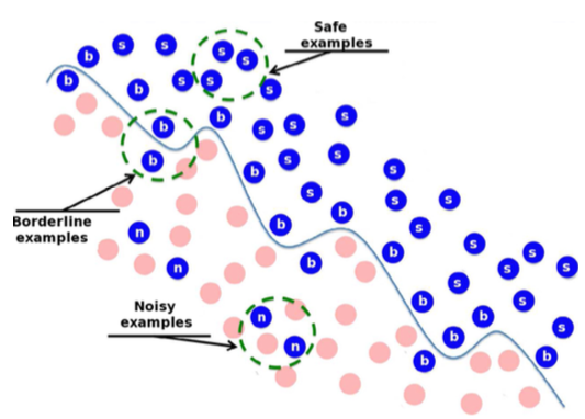
- Safe examples are placed in relatively homogeneous areas with respect to the class label.
- Borderline examples are located in the area surrounding class boundaries, where either the minority and majority classes overlap or these examples are very close to the difficult shape of the boundary.
- Noisy examples are individuals from one class occurring in the safe areas of the other class.
The examples belonging to the last two groups often do not contribute to a correct class prediction, and one could ask whether removing them could improve classification performance. In order to achieve this goal, this paper proposes combining SMOTE along with the noise filter IPF, claiming that:
- The SMOTE algorithm fulfills a dual function: it balances the class distribution and it helps to fill in the interior of sub-parts of the minority class.
- The IPF filter removes the noisy examples originally present in the dataset and also those created by SMOTE. Besides this, IPF cleans up the boundaries of the classes, making them more regular.
Synthetic imbalanced datasets with different shapes of the minority class, imbalance ratios and levels of borderline examples have been considered. A set of real-world imbalanced datasets with different quantities of noisy and borderline examples and other factors have been also considered. Additional noise has been introduced into the latter considering two noise schemes: a class noise scheme and an attribute noise scheme. You can download all these datasets from here:
- Synthetic Datasets

- Real-world Datasets
All these datasets have been preprocessed with our proposal and several re-sampling techniques that can be found in the literature:
- SMOTE in its basic version. The implementation of SMOTE used in this paper considers 5 nearest neighbors, the HVDM metric to compute the distance between examples and balances both classes to 50%.
- SMOTE + Tomek Links. This method uses tomek links (TL) to remove examples after applying SMOTE, which are considered being noisy or lying in the decision border. A tomek link is defined as a pair of examples x and y from different classes, that there exists no example z such that d(x,z) is lower than d(x,y) or d(y,z) is lower than d(x,y), where d is the distance metric.
- SMOTE-ENN. ENN tends to remove more examples than the TL does, so it is expected that it will provide a more in depth data cleaning. ENN is used to remove examples from both classes. Thus, any example that is misclassified by its three nearest neighbors is removed from the training set.
- SL-SMOTE. This method assigns each positive example its so called safe level before generating synthetic examples. The safe level of one example is defined as the number of positive instances among its k nearest neighbors. Each synthetic example is positioned closer to the example with the largest safe level so all synthetic examples are generated only in safe regions.
- Borderline-SMOTE. This method only oversamples or strengthens the borderline minority examples. First, it finds out the borderline minority examples P, defined as the examples of the minority class with more than half, but not all, of their m nearest neighbors belonging to the majority class. Finally, for each of those examples, we calculate its k nearest neighbors from P (for the algorithm version B1-SMOTE) or from all the training data, also with majority examples (for the algorithm version B2-SMOTE) and operate similarly to SMOTE. Then, synthetic examples are generated from them and added to the original training set.
Finally, several classification algorithms have been tested over these preprocessed datasets:
- C4.5 is a decision tree generating algorithm. It has been used in many recent analyses of imbalanced data. It induces classification rules in the form of decision trees from a set of given examples. The decision tree is constructed in a top-down way, using the normalized information gain (difference in entropy) that results from choosing an attribute to split the data. The attribute with the highest normalized information gain is the one used to make the decision.
- k-Nearest Neighbors (k-NN) finds a group of k instances in the training set that are closest to the test pattern. The predicted class label is based on the predominance of a particular class in this neighborhood. The distance and the number of neighbors are key elements of this algorithm.
- Support Vector Machine (SVM) maps the original input space into a high-dimensional feature space via a certain kernel function (avoiding the computation of the inner product of two vectors). In the new feature space, the optimal separating hyperplane with maximal margin is determined in order to minimize an upper bound of the expected risk instead of the empirical risk. We use SMO training algorithm to obtain the SVM classifiers.
- Repeated Incremental Pruning to Produce Error Reduction (RIPPER) builds a decision list of rules to predict the corresponding class for each instance. The list of rules is grown one by one and immediately pruned. Once a decision list for a given class is completely learned, an optimization stage is performed.
- PART is based on C4.5 algorithm. In each iteration, a partial C45 tree is generated and its best rule extracted (the one wich cover more examples). The algorithm ends when all the examples are covered. A partial tree is one whose braches are not fully explored. When a node has grown all its children, the node is eligible to prune. If the node is not pruned, all the exploration ends.
The classification algorithms have been executed using the parameters shown in the following table:
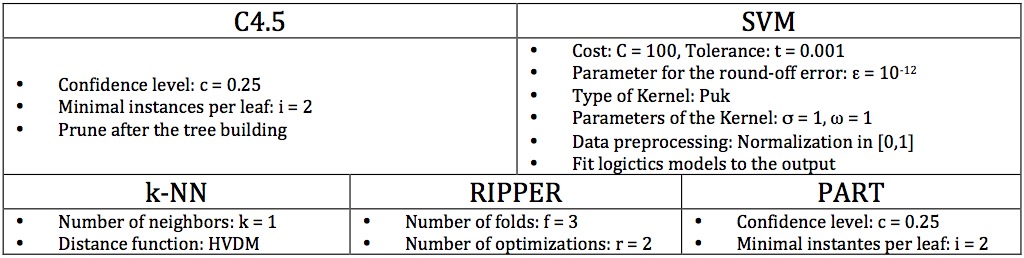
The implementation can be found in the KEEL Software Tool
The values of the AUC measure for C4.5 have shown that our proposal has a notably better performance when dealing with imbalanced datasets with noisy and borderline examples with both synthetic and real-world datasets. SMOTE-IPF also outperforms the rest of the methods with the real-world datasets with additional noise. Our proposal especially outperforms the rest of the methods with the more complex to learn datasets in each group of datasets: the non-linear synthetic datasets and the attribute noise real-world datasets. These observations are supported by statistical tests.
The experiments performed with others classifiers (k-NN, SVM, RIPPER and PART) have provided similar results and conclusions on the superiority of SMOTE-IPF to those for C4.5. Although statistical differences are less significant using SVM and RIPPER with attribute noise datasets, SMOTE-IPF obtains the better performances and the aligned Friedman's ranks. The especially good results of SMOTE-IPF on the synthetic datasets using RIPPER and on the class noise datasets using k-NN must also be pointed out. These results have been better than those of C4.5. The full results of the experimentation can be downloaded in the following table:
| Datasets | C4.5 | k-NN | SVM | RIPPER | PART |
|---|---|---|---|---|---|
| Synthetic | |||||
| Real-world | |||||
| Class Noise - 20% | |||||
| Class Noise - 40% | |||||
| Attribute Noise - 20% | |||||
| Attribute Noise - 40% |
INFFC: An iterative class noise filter based on the fusion of classifiers with noise sensitivity control
- José A. Sáez, M. Galar, J. Luengo, F. Herrera, INFFC: An iterative class noise filter based on the fusion of classifiers with noise sensitivity control. Information Fusion, 27 (2016) 19-32, doi: 10.1016/j.inffus.2015.04.002.
As previously commented, noise filters are widely used due to their benefits in the learning in terms of classification accuracy and complexity reduction of the models built. The study of the noise filtering schemes that are proposed in the literature focuses our attention on three main paradigms:
- Ensemble-based filtering. The main advantage of these approaches is based on the hypothesis that collecting predictions from different classifiers could provide a better class noise detection than collecting information from a single classifier.
- Iterative filtering. The strength of these types of filters is the usage of an iterative elimination of noisy examples under the idea that the examples removed in one iteration do not influence the noise detection in subsequent ones.
- Metric-based filtering. These noise filters are based on the computation of measures over the training data and usually allow the practitioner to control the level of conservation of the filtering in such a way that only examples whose estimated noise level exceed a prefixed threshold are removed.
On this account, this paper proposes a novel noise filtering technique combining these three noise filtering paradigms. In this way, we take advantage of the three different aforementioned paradigms. The proposal of this paper removes noisy examples in multiple iterations considering filtering techniques based on the usage of multiple classifiers. For this reason, we have called our proposal Iterative Noise Filter based on the Fusion of Classifiers (INFFC). Next figure shows an scheme of the filtering method proposed. Three steps are carried out in each iteration:
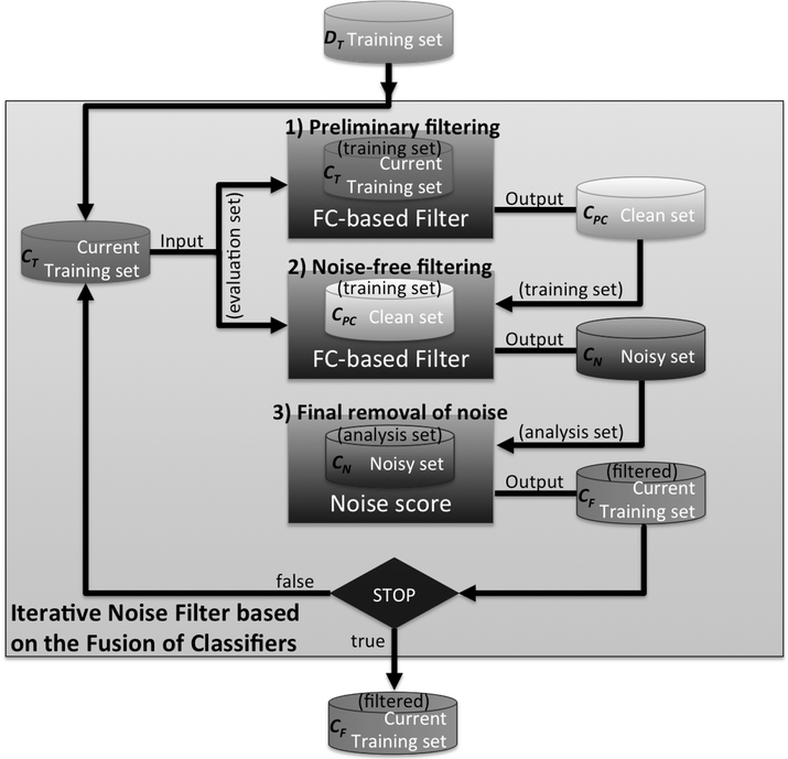
- Preliminary filtering. This first step removes a part of the existing noise in the current iteration to reduce its influence in posterior steps. More specifically, noise examples identified with high confidence are expected to be removed in this step.
- Noise-free filtering. A new filtering, which is built from the partially clean data from the previous step, is applied over all the training examples in the current iteration resulting into two sets of examples: a clean and a noisy set. This filtering is expected to be more accurate than the previous one since the noise filters are built from cleaner data.
- Final removal of noise. A noise score is computed over each potentially noisy example from the noisy set obtained in the previous step in order to determine which ones are finally eliminated.
A thorough empirical study will be developed comparing several representative noise filters (such as AllKNN, CF, ENN, ME, NCNE, EF, IPF) with our proposal. All of them will be used to preprocess the 25 real-world datasets (which are shown in the following table) in which different class noise levels will be introduced (from 5% to 30%, by increments of 5%).
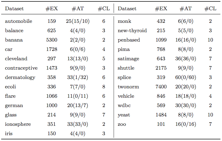
You can also download all these datasets by clicking here: ![]()
The filtered datasets will be then used to create classifiers with three learning methods of a different and well-known behavior against noise: C4.5, SVM and NN. Their test accuracy over the datasets preprocessed with our proposal and the other existing filters will be compared using the appropriate statistical tests in order to check the significance of the differences found. Furthermore, we analyze the examples removed by each one of the noise filters. In the following table you can download the files with the results of each method considered and the analysis of the examples affected by our proposal.
| Accuracy | Examples |
|---|---|
The most remarkable fact behind the analysis of results is that almost all the filters studied in this paper eliminate higher amounts of clean examples compared to INFFC. However, INFFC maintains a similar elimination level of noisy examples than that of other noise filters, particularly when the noise level increases. Thus our method is able to maintain a good balance between the examples that one must delete (noisy examples) and those that must not (clean examples). Furthermore, from the experimental results we can conclude that our noise filter enhance the performance of the rest of the noise filters and no preprocessing. The statistical analysis performed supports our conclusions.
Noise filtering efficacy prediction by data complexity measures
- José A. Sáez, J. Luengo, F. Herrera, Predicting Noise Filtering Efficacy with Data Complexity Measures for Nearest Neighbor Classification. Pattern Recognition, 46:1 (2013) 355-364, doi: 10.1016/j.patcog.2012.07.009.
Classifier performance, particularly of instance-based learners such as k-Nearest Neighbors, is affected by the presence of noisy data. In order to improve the classification performance of noise-sensitive methods when dealing with noisy data, noise filters are commonly applied. Their aim is to remove potentially noisy examples before building the classifier. However, both correct examples and examples containing valuable information can also be removed. This fact implies that these techniques do not always provide an improvement in performance. The success of these methods depends on several circumstances, such as the kind and nature of the data errors, the quantity of noise removed or the capabilities of the classifier to deal with the loss of useful information related to the filtering. Therefore, the efficacy of noise filters, i.e., whether their usage causes an improvement in classifier performance, depends on the noise-robustness and the generalization capabilities of the classifier used, but it also strongly depends on the characteristics of the data.
Data complexity measures are a recent proposal to represent characteristics of the data which are considered difficult in classification tasks, e.g., the overlapping among classes, their separability or the linearity of the decision boundaries.
This paper proposes the computation of these data complexity measures to predict in advance when the usage of a noise filter will statistically improve the results of a noise-sensitive learner: the nearest neighbor classifier (1-NN).
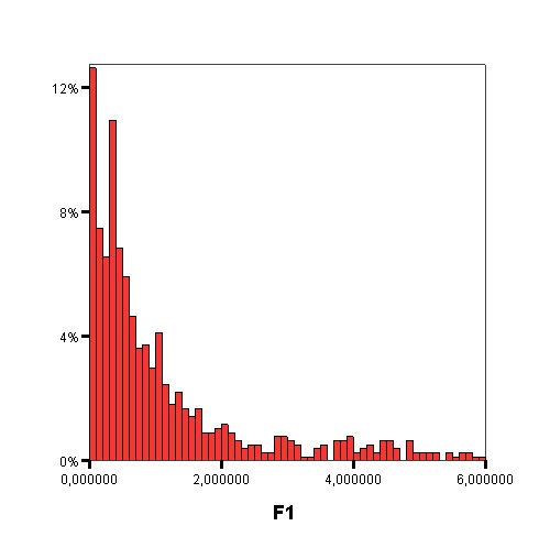
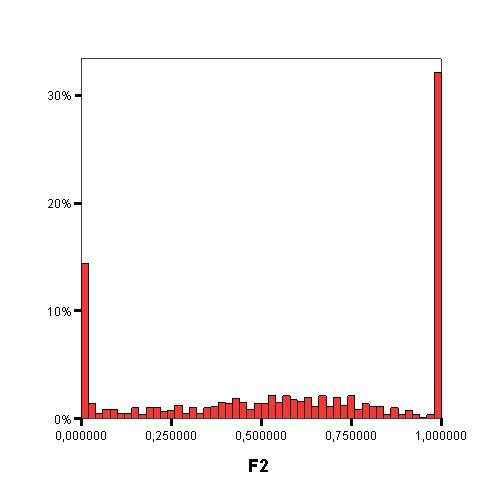
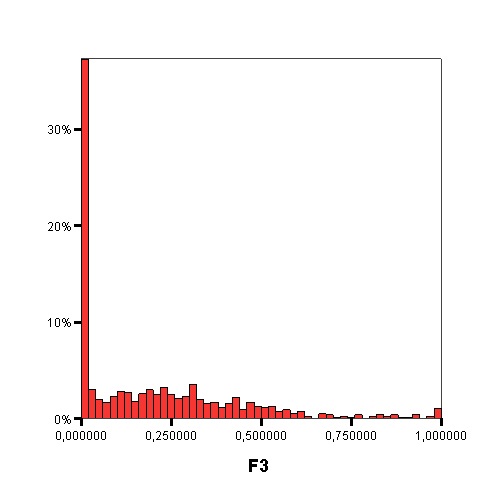
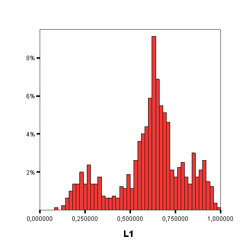
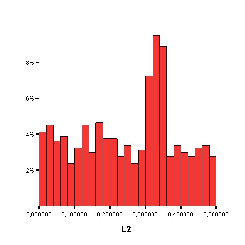
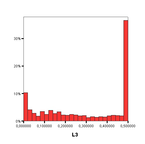
This paper considers the following 11 data complexity measures:
Measures of class overlapping: F1 - Maximum Fisher's discriminant ratio, F2 - Volume of the overlapping region, F3 - Maximum feature efficiency.
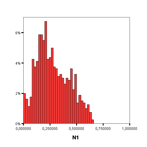
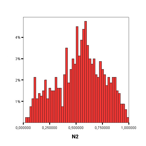
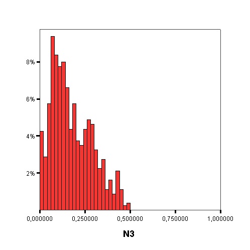
Measures of separability of classes: L1 - Minimized sum of error distance by linear programming, L2 - Error rate of linear classifier by linear programming, N1 - Rate of points connected to the opposite class by a minimum spanning tree, N2 - Ratio of average intra/inter class nearest neighbor distance, N3 - Error rate of the 1-NN classifier.
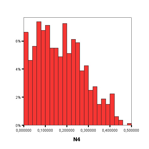
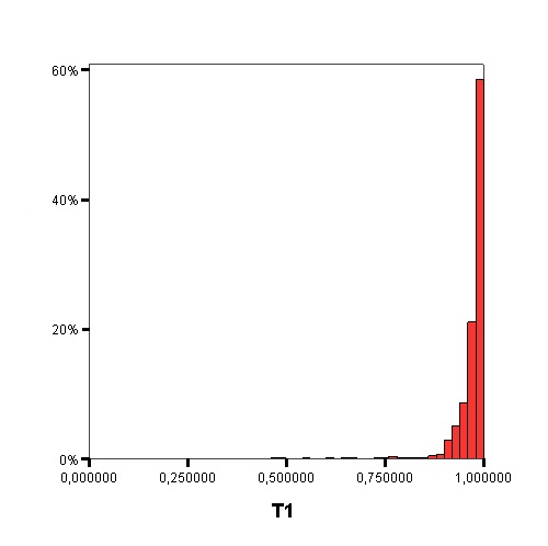
Measures of geometry, topology, and density of manifolds: L3 - Nonlinearity of a linear classifier by linear programming, N4 - Nonlinearity of the 1-NN classifier, T1 - Ratio of the number of hyperspheres, given by ε-neighborhoods, by the total number of points.
Noise filters are preprocessing mechanisms designed to detect and eliminate noisy examples in the training set. The result of noise elimination in preprocessing is a reduced and improved training set which is then used as an input to a machine learning algorithm. The noise filters analyzed in this paper are shown in the following table. They have been chosen due to their good behavior with many real-world problems.
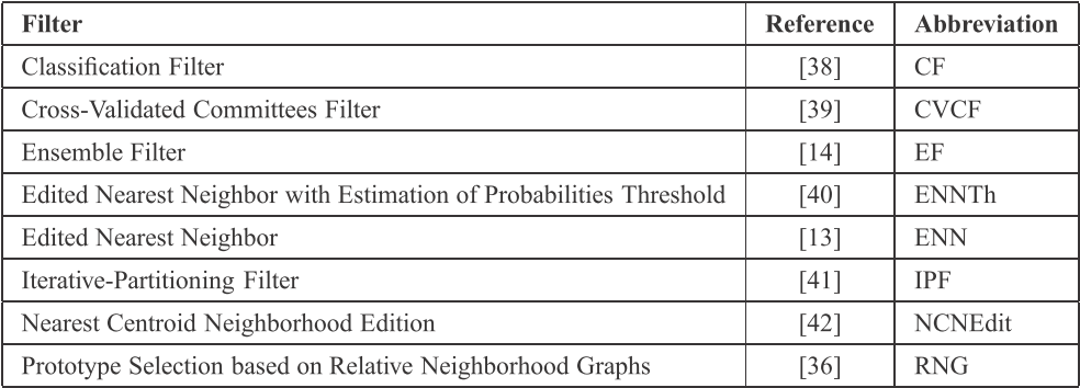
The implementation of these methods can be found in the KEEL Software Tool
We pretend to provide a rule set based on the characteristics of the data which enables one to predict whether the usage of noise filters will be statistically beneficial. Because of this, the methodology shown in the following figure has been designed.
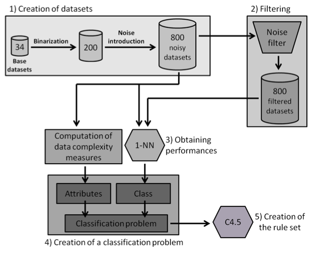
The complete process is described below:
- 800 different binary classification datasets are built from 34 base datasets. Several levels of random attribute noise (0%, 5%, 10% and 15%) are introduced into them.
The 34 base datasets are shown in the following table. They have been selected from the KEEL-dataset repository.
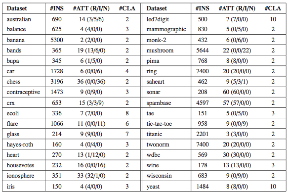
You can download the binary datasets created by clicking here: ZIP file
- These 800 datasets are filtered with a noise filter, leading to 800 new filtered datasets.
- The test performance of 1-NN on each of the 800 datasets, both with and without the application of the noise filter, is computed. The estimation of the classifier performance is obtained by means of 3 runs of a 10-fold cross-validation and their results are averaged. The AUC metric is used due it being commonly employed when working with binary datasets and the fact that it is less sensitive to class imbalance. The performance estimation is used to check which datasets are improved in their performance by 1-NN when using the noise filter. The results of 1-NN -with and without filtering can be checked here:
- A classification problem is created with each example being one of the datasets built and in which:
- (i) the attributes are the 11 data complexity metrics for each dataset.
- (ii) the class label represents whether the usage of the noise filter implies a statistically significant improvement of the test performance. Wilcoxon's statistical test -with a significance level of 0.1- is applied to compare the performance results of the 3x10 test folds with and without the usage of the noise filter. Depending on whether the usage of the noise filter is statistically better than the lack of filtering, each example is labeled as positive or negative, respectively.
The file with the values of each data complexity measure can be downloaded here: XLS file

The following graphics show the histograms representing the distribution of values of each data complexity metric. The size of each interval is 0.1 for the F1 metric and 0.02 for the rest of measures.
- Finally, similarly to the method of Orriols-Puig and Casillas, the C4.5 algorithm is used to build a decision tree on the aforementioned classification problem, which can be transformed into a rule set. The performance estimation of this rule set is obtained using a 10-fold cross-validation. By means of the analysis of the decision trees built by C4.5, it is possible to check which are the most important data complexity metrics to predict the noise filtering efficacy, i.e., those in the top levels of the tree and appearing more times, and their performance examining the test results.
The procedure described above has been followed with each one of the noise filters. The following table shows the performance results of the rule sets obtained with C4.5 on the training and test sets for each noise filter when predicting the noise filtering efficacy, i.e., when discriminating between the aforementioned positive and negative classes.
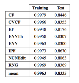
These results obtained have shown that there is a notable relation between the characteristics of the data and the efficacy of several noise filters, as the rule sets have good prediction performances.
Studying the order, from 1 to 11, in which the first node corresponding with each data complexity metric appears in the decision tree, starting from the root and the percentage of nodes of each data complexity metric in the decision tree it is possible to check that the most influential metrics are F2, N2, F3 and T1.
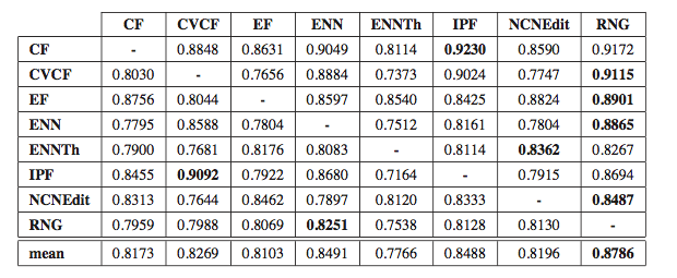
Considering these 4 metrics, we learn rules to predict the behavior of one filter and this is tested to predict the behavior of the rest of the noise filters (see the following table). From these results, the prediction performance of the rules learned for the RNG filter is clearly the more general, since they are applicable to the rest of the noise filters obtaining the best prediction results -see the last column with an average of 0.8786. Therefore, this rule set has rules that are more similar to the rest of the noise filters and thus, it represents better the common characteristics on which the efficacy of all noise filters depends. This shows that the conditions under which a noise filter works well are similar for other noise filters.
The final rule set proposed to predict the noise filtering efficacy of all the noise filters is therefore the following:
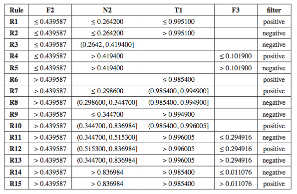
The analysis of the rules that are triggered more often predicting the behavior of the different noise filters shows that, generally, noise filtering statistically improves the classifier performance of the nearest neighbor classifier when dealing with problems with a high value of overlapping among the classes. However, if the problem has several clusters with a low overlapping among them, noise filtering is generally unnecessary and can indeed cause the classification performance to deteriorate.
Quantifying the benefits of using MCS with noise
José A. Sáez, M. Galar, J. Luengo, F. Herrera, Tackling the Problem of Classification with Noisy Data using Multiple Classifier Systems: Analysis of the Performance and Robustness. Information Sciences 247 (2013) 1-20, doi: 10.1016/j.ins.2013.06.002.
This paper analyzes how well several MCSs behave with noisy data by means the realization of a huge experimental study. In order to do this, both the performance and the noise-robustness of different MCSs have been compared with respect to their single classification algorithms. A large number of noisy datasets have been created considering different types, schemes and levels of noise to perform these comparisons.
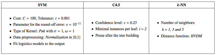
We consider as single classification algorithms SVM, C4.5 and k-NN. Considering the previous classifiers, the following MCS are built:
- MCS3-k. These MCSs are composed by 3 individual classifiers (SVM, C4.5 and k-NN). Three values of k are considered (1, 3 and 5), so we will create three different MCS3-k denoted as MCS3-1, MCS3-3 and MCS3-5.
- MCS5. This is composed by 5 different classifiers: SVM, C4.5 and k-NN with the 3 different values (1, 3 and 5).
- BagC4.5. This MCS considers C4.5 as baseline classifier.
Therefore, the MCSs built with heterogeneous classifiers (MCS3-k and MCS5) will contain a noise-robust algorithm (C4.5), a noise-sensitive method (SVM) and a method whose robustness varies depending on the value of k (k-NN). Hence, how the behavior of each MCS3-k and the MCS5 depends on that of each single method can be analyzed. In the case of BagC4.5, it is compared to its base classifier, that is, C4.5. The configuration parameters used to build the classifiers considered are shown in the following table. The same parameter setup for each classification algorithm, considered either as part of a MCS or individually, has been used for all the datasets. This will help us to know to what extent the same classifier trained with the same parameters over the same training data can imply an advantage incorporating it into a MCS with respect to its usage alone.
The experimentation is based on the forty real-world classification problems from the KEEL-dataset repository shown in the following table.
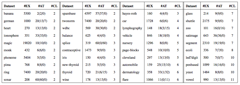
You can download these data sets by clicking here: ZIP file ![]()
A collection of noisy data sets are created from the aforementioned forty base data sets. Both types of noise are independently considered: class (the random and the paiwise schemes) and attribute (the random and the Gaussian schemes) noise. For each type of noise, the noise levels ranging from x = 0% (base datasets) to x = 50%, by increments of 5%, are studied.
You can download all these noisy data sets by clicking in the following links:
- ZIP file - Random class noise scheme
- ZIP file - Pairwise class noise scheme
- ZIP file - Random attribute noise scheme
- ZIP file - Gaussian attribute noise scheme
We will study the following four combination methods for the MCSs built with heterogeneous classifiers:
- Majority vote (MAJ). This is a simple but powerful approach, where each classifier gives a vote to the predicted class and the most voted one is chosen as the output.
- Weighted majority vote (W-MAJ). Similarly to MAJ, each classifier gives a vote for the predicted class, but in this case, the vote is weighted depending on the competence (accuracy) of the classifier in the training phase.
- Naive Bayes (NB). This method assumes that the base classifiers are mutually independent. Hence, the predicted class is that one obtaining the highest posterior probability. In order to compute these probabilities, the confusion matrix of each classifier is considered.
- Behavior-Knowledge Space (BKS). This is a multinomial method that indexes a cell in a look-up table for each possible combination of classifiers outputs. A cell is labeled with the class to which the majority of the instances in that cell belong to. A new instance is classified by the corresponding cell label; in case that for the cell is not labeled or there is a tie, the output is given by MAJ.
In order to check the behavior of the different methods when dealing with noisy data, the results of each MCS are compared with those of their individual components using two distinct properties:
- The performance of the classification algorithms on the test sets for each level of induced noise, defined as its accuracy rate.
- The robustness of each method is estimated with the relative loss of accuracy (RLA)
In order to properly analyze the performance and RLA results, Wilcoxon's signed rank statistical test is used. This is a non-parametric pairwise test that aims to detect significant differences between two sample means; that is, between the behavior of the two algorithms involved in each comparison. For each type and noise level, the MCS and each single classifier will be compared using Wilcoxon's test and the p-values associated with these comparisons will be obtained. The p-value represents the lowest level of significance of a hypothesis that results in a rejection and it allows one to know whether two algorithms are significantly different and the degree of this difference. Both performance and robustness are studied because the conclusions reached with one of these metrics need not imply the same conclusions with the other.
The results obtained by the different methods can be downloaded in the following links:
| Base | MAJ | W-MAJ | NB | BKS | BagC4.5 |
|---|---|---|---|---|---|
The results obtained have shown that the MCSs studied do not always significantly improve the performance of their single classification algorithms when dealing with noisy data, although they do in the majority of cases (if the individual components are not heavily affected by noise). The improvement depends on many factors, such as the type and level of noise. Moreover, the performance of the MCSs built with heterogeneous classifiers depends on the performance of their single classifiers, so it is recommended that one studies the behavior of each single classifier before building the MCS. Generally, the MCSs studied are more suitable for class noise than for attribute noise. Particularly, they perform better with the most disruptive class noise scheme (uniform one) and with the least disruptive attribute noise scheme (Gaussian one). However, BagC4.5 works well with both types of noise, with the exception of the pairwise class noise, where its results are not as accurate as with other types of noise.
The robustness results show that the studied MCS built with heterogeneous classifiers will not be more robust than the most robust among their single classification algorithms. In fact, the robustness can always be shown as an average of the robustnesses of the individual methods. The higher the robustnesses of the individual classifiers are, the higher the robustness of the MCS is. Nevertheless, BagC4.5 is again an exception: it becomes more robust than its single classifier C4.5.
The study of several decisions combination methods show that the majority vote scheme is a simple yet powerful alternative to other techniques when working with noisy data.
Advantages of OVO scheme in the presence of noise
José A. Sáez, M. Galar, J. Luengo, F. Herrera, Analyzing the Presence of Noise in Multi-class Problems: Alleviating its Influence with the One-vs-One Decomposition. Knowledge and Information Systems, 38:1 (2014) 179-206, doi: 10.1007/s10115-012-0570-1.
This paper analyzes the suitability of the usage of the OVO decomposition when dealing with noisy training datasets in multi-class problems.
The experimentation of this paper is based on twenty real-world multi-class classification problems from the KEEL dataset repository. Next table shows the datasets sorted by the number of classes (#CLA).
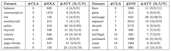
You can download these data sets by clicking here: ZIP file ![]()
A large collection of noisy data sets are created from the aforementioned 20 base data sets. Both types of noise are independently considered: class and attribute noise. For each type of noise, the noise levels ranging from x = 0% (base datasets) to x = 50%, by increments of 5%, are studied.
You can download all these noisy data sets by clicking in the following links:
- ZIP file - Random class noise scheme
- ZIP file - Pairwise class noise scheme
- ZIP file - Random attribute noise scheme
- ZIP file - Gaussian attribute noise scheme
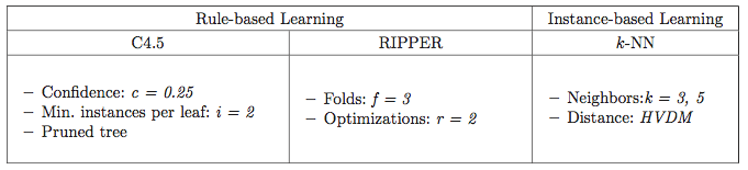
The C4.5 and RIPPER robust learners and the noise-sensitive k-NN method have been evaluated on these datasets, with and without the usage of OVO. The classification algorithms have been executed using the default parameters recommended by the authors, which are shown in the following table.
The results obtained by the different methods can be downloaded in the following links:
| Class Noise | Accuracy | Robustness |
|---|---|---|
| Random | ||
| Pairwise |
| Attribute Noise | Accuracy | Robustness |
|---|---|---|
| Random | ||
| Gaussian |
The results obtained have shown that the OVO decomposition improves the baseline classifiers in terms of accuracy when data is corrupted by noise in all the noise schemes studied.
The robustness results are particularly notable with the more disruptive noise schemes - the random class noise scheme and the random attribute noise scheme - where a larger amount of noisy examples and with higher corruptions are available, which produces greater differences (with statistical significance).
Three hypotheses could be introduced aiming to explain the better performance and robustness of the methods using OVO when dealing with noisy data: (i) the distribution of the noisy examples in the subproblems, (ii) the increase of the separability of the classes and (iii) the possibility of collecting information from different classifiers.
As final remark, we must emphasize that one usually does not know the type and level of noise present in the data of the problem that is going to be addressed. Decomposing a problem suffering from noise with OVO has shown a better accuracy, higher robustness and homogeneity with all the classification algorithms tested. For this reason, the usage of the OVO decomposition strategy in noisy environments can be recommended as an easy-to-applicate, yet powerful tool to overcome the negative effects of noise in multi-class problems.
Using the One-vs-One decomposition to improve the performance of class noise filters
L.P.F. Garcia, J.A. Sáez, J. Luengo, A.C. Lorena, A.C.P.L.F. de Carvalho, F. Herrera, Using the One-vs-One decomposition to improve the performance of class noise filters via an aggregation strategy in multi-class classification problems. Knowledge-Based Systems, 90 (2015) 153-164, doi: 10.1016/j.knosys.2015.09.023.
The behavior of the OVO strategy in presence of noise was studied in "Advantages of OVO scheme in the presence of noise". This paper investigates a new approach to detect and remove label noise in multi-class classification tasks. This approach combines the OVO multi-class decomposition strategy with a group of noise filtering techniques. In this combination, each noise filter, instead of being applied to the original multi-class dataset, is applied to each binary subproblem produced by the OVO strategy. Each noise filter assigns to each training instance a degree of confidence of the example being noisy, named noise degree prediction (NDP), which is a real number.
The NDPs obtained from all noise filters are combined using a soft voting strategy, producing a unique NDP for the instance. The strategy adopted in this paper is to remove a fixed number of the examples with highest NDP values. The proposed approach has three main advantages:
- it does not require any modification in the concept and the bias of the noise filters;
- it provides for each training instance a combined degree of confidence regarding noise identification and;
- it does not make any assumptions about the noise characteristics.
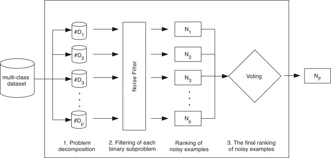
The proposal is composed of three main steps:
- Problem decomposition. In this phase, the multi-class classification problem is decomposed into p binary subproblems using the OVO decomposition strategy.
- Filtering of each binary subproblem. When using decomposition for classification purposes, a classifier is built for each one of the p binary subproblems. Similarly, our proposal applies a noise filter to each one of the subproblems created in the previous step. Since the noise filters are adapted to output a confidence level regarding the noise predictions (the NDP values), this step results in p different lists of NDP values (N1,…,Np), each one with the NDP values of the examples belonging to the binary subproblem in which the filter is applied.
- Combination of the lists of noisy examples. In the same way that the predictions of the different classifiers must be combined when using decomposition for classification, our proposal also requires a last step where the different lists of NDP values (N1,…,Np) are combined. Thus, a unique final list of NDP values (NF), which will be ordered from the highest to lowest value (from the noisiest example to the cleanest example), is computed in this last step. For the combination of these lists, the average NDP of each example is computed.
These steps are summarized in the following figure.
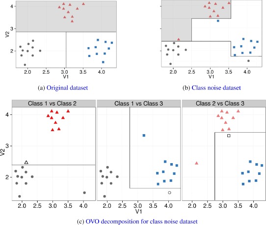
By means of this OVO decomposition, the base filters can be more effective. Since the decomposition of the multi-class problem can create simpler subproblems (with a higher degree of separation between the classes) and distributes the noisy examples in several subproblems, the noise filters can improve their detection capabilities when compared with preprocessing the original multi-class dataset. The following figure illustrates how by decomposing the problem, the class border become simpler and thus the filtering task can be more effective.
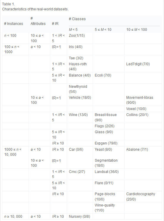
In the paper we analyze the suitability of this proposal compared to several filters. 28 multi-class classification datasets were used as shown in the following table with their characteristics.
In order to assess the performance of the noise filtering scheme proposed, the behavior of each one of the five aforementioned noise filters for the multi-class and decomposed problems was measured. The ability of the filters in noise detection is recorded in both scenarios. Finally, the performance achieved by the filters in noise retrieval for the multi-class and decomposed subproblems are compared.
The precision at N (p@N) metric is used. Thereby, N is a threshold on the number of examples in NF that will be regarded as noisy. We set N to be the number of noisy examples artificially introduced in the datasets, as in [47]. The precision in noise detection is then defined as the number of correctly identified noisy cases (#correct_noisy#correct_noisy) divided by the number of examples identified by the filter as noisy (the threshold N):
The average p@N values obtained by the filters in the identification of the artificial noise inserted are shown in the heatmap of the following figure. There are two groups of columns in this figure, one for each type of strategy: (1) using the original multi-class datasets and (2) using the datasets decomposed by the OVO strategy. Each column represents one filter, while each row corresponds to a specific dataset. While higher p@N values are colored in green scale, lower p@N score levels are colored in blue scale.
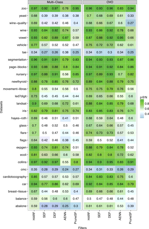
Further analysis were also carried out. For each noise level, the performance of the filters is shown as follows. In general, for all datasets there are at least three filters with improved performance. While SEF, DEF and PruneSF had their performance improved for low noise levels, AENN showed improved results for high noise levels. The HARF filter had improved performance for high noise levels, but mostly it was not significant. There is a specific dataset where most of the filters achieved a low performance when OVO was employed: balance. In the datasets collins, expgen, flags and tae the results were impaired for specific noise levels. Except for the dataset expgen, most of the previous datasets are imbalanced.

The effect of the OVO strategy for filtering in imbalanced data sets was also analyzed. The figure presented below shows the evolution of the Imbalanced Ratio (IR) of the filtered data sets as the introduced noise increases.
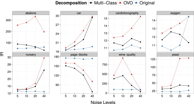
The OVO strategy presents the largest changes of IR for the datasets abalone, for all noise levels, wine-quality for 10% of noise level, and yeast for 20 and 40% of noise level. Even when improved the performance, OVO always increased the imbalance in the datasets and tended to remove more minority class examples. This is a harmful effect that can be due to the several filter application to each example in the OVO strategy, increasing its probability of being labeled as noisy. Nonetheless, the increase of IR seems to be a harmful effect of noise pre-processing, despite the filtering scheme employed. Some strategies can minimize these effects, such as weight the NDP of an example by the proportion of training examples from its class. This could decrease the reduction of the minority class examples by the filters.
To sum up, the OVO decomposition presented a better performance than the multi-class strategy in almost all analysis carried out. This may have occurred because, while in the original multi-class dataset the information has a complex structure representation, the simpler structure of the binary subproblems after the OVO decomposition helps the identification of the noisy data.
Results from a separate analysis in imbalanced datasets showed that filtering tends to increase the imbalance, regardless of the filtering scheme employed. OVO intensified this effect. These results should be further investigated, taking into account the performance of the filters in the individual classes. This analysis also reinforced the importance of the presence of a domain specialist to analyze the results, even when the noise filters show a good performance in the overall noise identification task.
Datasets used
All the datasets used in the papers about noisy data that are detailed above have been taken from the KEEL dataset repository. Next table contains direct links to the datasets used in each one of the papers:
| Paper | Datasets |
|---|---|
| José A. Sáez, J. Luengo, F. Herrera, Predicting Noise Filtering Efficacy with Data Complexity Measures for Nearest Neighbor Classification. Pattern Recognition, 46:1 (2013) 355-364, doi: 10.1016/j.patcog.2012.07.009. |
Datasets |
| José A. Sáez, M. Galar, J. Luengo, F. Herrera, INFFC: An iterative class noise filter based on the fusion of classifiers with noise sensitivity control. Information Fusion, 27 (2016) 19-32, doi: 10.1016/j.inffus.2015.04.002. |
Datasets |
| José A. Sáez, J. Luengo, J. Stefanowski, F. Herrera, SMOTE–IPF: Addressing the noisy and borderline examples problem in imbalanced classification by a re-sampling method with filtering. Information Sciences, 291 (2015) 184-203, doi: 10.1016/j.ins.2014.08.051. |
|
| José A. Sáez, M. Galar, J. Luengo, F. Herrera, Tackling the Problem of Classification with Noisy Data using Multiple Classifier Systems: Analysis of the Performance and Robustness. Information Sciences 247 (2013) 1-20, doi: 10.1016/j.ins.2013.06.002. |
|
| José A. Sáez, M. Galar, J. Luengo, F. Herrera, Analyzing the Presence of Noise in Multi-class Problems: Alleviating its Influence with the One-vs-One Decomposition. Knowledge and Information Systems, 38:1 (2014) 179-206, doi: 10.1007/s10115-012-0570-1. |
Noise Data Software
We have developed a R package available in CRAN named NoiseFiltersR, which contains a large selection of noise filters to deal with class noise in a friendly, unified manner.
The included filters are among several types as shown in the next table:

Installation
The NoiseFiltersR package is available at CRAN servers, so it can be downloaded and installed directly from the R command line by typing:
> install.packages("NoiseFiltersR")
This command will also install the eleven dependencies of the package, which mainly provide the classification algorithms needed for some of the implemented filters, and which can be looked up in the “Imports” section of the CRAN website for the package.
In order to easily access all the package’s functions, it must be attached in the usual way:
> library(NoiseFiltersR)
Documentation
The Rjournal paper on the NoiseFiltersR package contains all the tips and helpful hints on how to use the package:
- Pablo Morales, Julián Luengo, Luís P.F. Garcia, Ana C. Lorena, André C.P.L.F. de Carvalho and Francisco Herrera, The NoiseFiltersR Package: Label Noise Preprocessing in R. RJournal, in press (2017).
Bibliography compilation about noise in data mining
We have performed a bibliography compilation of journal papers on Noise in Data Mining. It is maintained by José A. Sáez.