
Analysing the Classification of Imbalanced Data-sets with Multiple Classes: Binarization Techniques and Ad-Hoc Approaches for Preprocessing and Cost Sensitive Learning
This Website contains additional material to the paper
A. Fernández, V. López, M. Galar, M.J. del Jesus and F. Herrera, Analysing the Classification of Imbalanced Data-sets with Multiple Classes: Binarization Techniques and Ad-Hoc Approaches for Preprocessing and Cost Sensitive Learning. Submitted to Knowledge Based Systems Journal, according to the following summary:
- Paper Content
- Description of the Algorithms Selected in the Paper
- Data-sets partitions Employed in the Paper
- Experimental Study
Paper Content
A. Fernández, V. López, M. Galar, M.J. del Jesus and F. Herrera, Analysing the Classification of Imbalanced Data-sets with Multiple Classes: Binarization Techniques and Ad-Hoc Approaches for Preprocessing and Cost Sensitive Learning. Submitted to Knowledge Based Systems Journal, according to the following summary:
Abstract: Within the real world applications of classification in engineering, there is a type of problem which is characterised by having a very different distribution of examples among their classes. This situation is known as the imbalanced class problem and it creates a handicap for the correct identification of the different concepts that are required to be learnt.
Traditionally, researches have addressed the binary class imbalanced problem, where there is a positive and a negative class. In this work, we aim to go one step further focusing our attention on those problems with multiple imbalanced classes. This condition imposes a harder restriction when the objective of the final system is to obtain the most accurate precision for each one of the different classes of the problem.
The goal of this work is to provide a throughout experimental analysis that will allow us to determine the behaviour of different approaches proposed in the specialized literature. First, we will make use of binarization schemes, i.e. one-vs-one and one-vs-all, in order to apply the standard approaches for solving binary class imbalanced problems. Second, we will apply several procedures which have been designed ad-hoc for the scenario of imbalanced data-sets with multiple classes.
This experimental study will include several well-known algorithms from the literature such as Decision Trees, Support Vector Machines and Instance-Based Learning, trying to obtain a global conclusion from different classification paradigms. The extracted findings will be supported by a statistical comparative analysis under more than 20 data-sets from the KEEL repository.
Summary:
- Introduction.
- Imbalanced Data-sets in Classification.
- The problem of imbalanced data-sets.
- Addressing the imbalanced problem: preprocessing and cost sensitive learning.
- Evaluation in imbalanced domains.
- Solving Multiple Class Imbalanced Data-sets.
- Static-SMOTE.
- Global-CS.
- Synergy of standard approaches for imbalanced data-sets and binarization techniques.
- One-vs-One approach.
- One-vs-All approach.
- Experimental Framework.
- Data-sets.
- Algorithms selected for the study.
- Web page associated to the paper.
- Experimental Study.
- Analysis of the combination of preprocessing and cost sensitive approaches with multi-classification.
- Study of the use of OVO versus OVA for imbalanced data-sets.
- Comparative analysis for pairwise learning with preprocessing/cost sensitive learning and standard approaches in multiple class imbalanced problems.
- C4.5 Decision Tree.
- Support Vector Machines.
- k-Nearest Neighbour.
- Lessons learned and future work.
- Concluding Remarks.
Description of the Algorithms Selected in the Paper
Preprocessing and Cost Sensitive Learning
A large number of approaches have previously been proposed to deal with the class imbalance problem, both for standard learning algorithms and for ensemble techniques (M. Galar, A. Fernández, E. Barrenechea, H. Bustince, and F. Herrera, "A review on ensembles for class imbalance problem: Bagging, boosting and hybrid based approaches," IEEE Trans. Syst., Man, Cybern. C, 2012). These approaches can be categorised in three groups:
Data level solutions: the objective consists in rebalancing the class distribution by sampling the data space to diminish the effect caused by their class imbalance acting as a external approach (N.V. Chawla, K. W. Bowyer, L. O. Hall, and W. P. Kegelmeyer, "Smote: Synthetic minority over-sampling technique," J. Artif. Intell. Res., vol. 16, pp. 321–357, 2002, G. E. A. P. A. Batista, R. C. Prati, and M. C. Monard, "A study of the behaviour of several methods for balancing machine learning training data," SIGKDD Explor. Newsl., vol. 6, no. 1, pp. 20–29, 2004., Y. Tang, Y.-Q. Zhang, and N. V. Chawla, "SVMs modeling for highly imbalanced classification,” IEEE Trans. Syst., Man, Cybern. B, vol. 39, no. 1, pp. 281–288, 2009.).
Algorithmic level solutions: these solutions try to adapt several classification algorithms to reinforce the learning towards the positive class. Therefore, they can be defined as internal approaches that create new algorithms or modify existing ones to take the class imbalance problem into consideration (B. Zadrozny and C. Elkan, “Learning and making decisions when costs and probabilities are both unknown,” in Proceedings of the 7th International Conference on Knowledge Discovery and Data Mining (KDD’01), 2001, pp. 204–213.,R. Barandela, J. S. Sánchez, V. García, and E. Rangel, “Strategies for learning in class imbalance problems,” Pattern Recogn., vol. 36, no. 3, pp. 849–851, 2003., C. Diamantini and D. Potena, “Bayes vector quantizer for class imbalance problem,” IEEE Trans. Knowl. Data Eng., vol. 21, no. 5, pp. 638–651, 2009.).
Cost sensitive solutions: this type of solutions incorporate approaches at the data level, at the algorithmic level, or at both levels jointly, considering higher costs for the misclassification of examples of, the positive class with respect to the negative class, and therefore, trying to minimise higher cost errors (P. Domingos, “Metacost: a general method for making classifiers cost sensitive,” in Advances in Neural Networks, International Journal of Pattern Recognition and Artificial Intelligence, 1999, pp. 155–164., K. M. Ting, “An instance-weighting method to induce cost-sensitive trees,” IEEE Trans. Knowl. Data Eng., vol. 14, no. 3, pp. 659–665, 2002., B. Zadrozny, J. Langford, and N. Abe, “Cost-sensitive learning by cost-proportionate example weighting,” in Proceedings of the 3rd IEEE International Conference on Data Mining (ICDM’03), 2003, pp. 435–442., Y. Sun, M. S. Kamel, A. K. C. Wong, and Y. Wang, “Cost-sensitive boosting for classification of imbalanced data,” Pattern Recogn., vol. 40, pp. 3358–3378, 2007., H. Zhao, “Instance weighting versus threshold adjusting for cost sensitive classification.” Knowl. Inf. Syst., vol. 15, no. 3, pp. 321–334, 2008., Z.-H. Zhou and X.-Y. Liu, “On multi-class cost-sensitive learning,” Comput. Intell., vol. 26, no. 3, pp. 232–257, 2010.).
The advantage of the data level solutions is that they are more versatile, since their use is independent of the classifier selected. Furthermore, we may preprocess all data-sets before-hand in order to use them to train different classifiers. In this manner, we only need to prepare the data once. There exists different rebalancing methods for preprocessing the training data, that can be classified into three groups:
Undersampling methods that create a subset of the original data-set by eliminating some of the examples of the majority class.
Oversampling methods that create a superset of the original data-set by replicating some of the examples of the minority class or creating new ones from the original minority class instances.
Hybrid methods that combine the two previous methods, eliminating some of the minority class examples expanded by the oversampling method in order to eliminate overfitting.
Regarding algorithmic level approaches, the idea is to choose an appropriate inductive bias given a specific classifier. Also, recognition-based one-class learning is used to model a system by using only the examples of the target class in the absence of the counter examples. This approach does not try to partition the hypothesis space with boundaries that separate positive and negative examples, but it attempts to make boundaries which surround the target concept, for example in SVMs.
Cost sensitive learning takes into account the variable cost of a misclassification of the different classes. The cost sensitive learning process tries to minimise the number of high cost errors and the total error of misclassification. Therefore, cost sensitive learning supposes that there is a cost matrix available for the different type of errors; however, given a data-set, this matrix is not usually given (Y. Sun, M. S. Kamel, A. K. C. Wong, and Y. Wang, “Cost-sensitive boosting for classification of imbalanced data,” Pattern Recogn., vol. 40, pp. 3358–3378, 2007.,Y. Sun, A. K. C. Wong, and M. S. Kamel, “Classification of imbalanced data: A review,” International Journal of Pattern Recognition and Artificial Intelligence, vol. 23, no. 4, pp. 687–719, 2009.).
In order to develop our experimental study, we have selected from the specialised literature several representative methods that deals with imbalanced classification for the aforementioned families. Specifically we have chosen four undersampling and four oversampling techniques, and a cost sensitive learning approach which are described below. We must also stress that all these mechanisms are available within the KEEL software tool http://www.keel.es (J. Alcalá-Fdez, L. Sánchez, S. García, M. J. del Jesus, S. Ventura, J. M. Garrell, J. Otero, C. Romero, J. Bacardit, V. M. Rivas, J. C. Fernández, and F. Herrera, “KEEL: A software tool to assess evolutionary algorithms to data mining problems,” Soft Comp., vol. 13, no. 3, pp. 307–318, 2009.).
Synthetic Minority Oversampling Technique (SMOTE) (N. V. Chawla, K. W. Bowyer, L. O. Hall, and W. P. Kegelmeyer, “Smote: Synthetic minority over-sampling technique,” J. Artif. Intell. Res., vol. 16, pp. 321–357, 2002.). Since the next two oversampling approaches are based on this technique, in what follows we will explain it in detail its main features.
With this approach, the positive class is over-sampled by taking each minority class sample and introducing synthetic examples along the line segments joining any/all of the k minority class nearest neighbours. Depending upon the amount of over-sampling required, neighbours from the k nearest neighbours are randomly chosen. This process is illustrated in the following Figure, where $x_i$ is the selected point, $x_i1$ to $x_i4$ are some selected nearest neighbours and $r_1$ to $r_4$ the synthetic data points created by the randomized interpolation. The implementation of this work uses only one nearest neighbour with the euclidean distance, and balances both classes to 50% distribution.
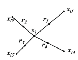
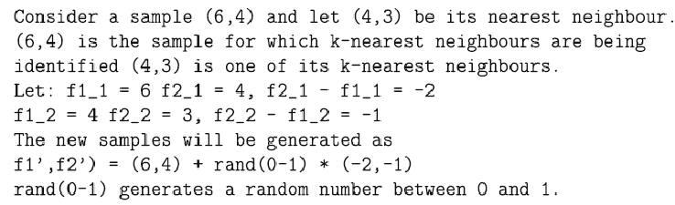
Synthetic samples are generated in the following way: Take the difference between the feature vector (sample) under consideration and its nearest neighbour. Multiply this difference by a random number between 0 and 1, and add it to the feature vector under consideration. This causes the selection of a random point along the line segment between two specific features. This approach effectively forces the decision region of the minority class to become more general. An example is detailed in the next Figure.
In short, the main idea is to form new minority class examples by interpolating between several minority class examples that lie together. In contrast with the common replication techniques (for example random oversampling), in which the decision region usually become more specific, with SMOTE the overfitting problem is somehow avoided by causing the decision boundaries for the minority class to be larger and to spread further into the majority class space, since it provides related minority class samples to learn from. Specifically, selecting a small k-value could also avoid the risk of including some noise in the data.
- SMOTE + Edited Nearest Neighbour (SMOTE+ENN) (G. E. A. P. A. Batista, R. C. Prati, and M. C. Monard, “A study of the behaviour of several methods for balancing machine learning training data,” SIGKDD Explor. Newsl., vol. 6, no. 1, pp. 20–29, 2004.). When applying SMOTE, class clusters may be not well defined in cases where some majority class examples invade the minority class space. The opposite can also be true, since interpolating minority class examples can expand the minority class clusters, introducing artificial minority class examples too deeply into the majority class space. Inducing a classifier in such a situation can lead to overfitting. For this reason, the ``SMOTE + ENN'' hybrid approach, applies the Wilson's ENN rule (D. Wilson, “Asymptotic properties of nearest neighbor rules using edited data,” IEEE Transactions on Systems, Man, and Communications, vol. 2, no. 3, pp. 408–421, 1972.) after the SMOTE application to remove from the training set any example misclassified by its three nearest neighbours.
- Safe-Level SMOTE (C. Bunkhumpornpat, K. Sinapiromsaran, and C. Lursinsap, “Safe-level- SMOTE: Safe-level-synthetic minority over-sampling TEchnique for handling the class imbalanced problem.” in Pacific-Asia Conference on Knowledge Discovery and Data Mining (PAKDD09), ser. Lecture Notes in Computer Science, T. Theeramunkong, B. Kijsirikul, N. Cercone, and T. B. Ho, Eds., vol. 5476. Springer, 2009, pp. 475–482.). As we described previously, SMOTE randomly synthesises the minority instances along a line joining a minority instance and its selected nearest neighbours, ignoring nearby majority instances. On the contrary, Safe-Level SMOTE carefully samples minority instances along the same line with different weight degree, called safe level. The safe level is computed by using k-nearest neighbour minority instances. Then, if the safe level of an instance is close to 0, the instance is nearly noise. If it is close to k, the instance is considered safe.
- Random-Oversampling (G. E. A. P. A. Batista, R. C. Prati, and M. C. Monard, “A study of the behaviour of several methods for balancing machine learning training data,” SIGKDD Explor. Newsl., vol. 6, no. 1, pp. 20–29, 2004.). It is a non-heuristic method that aims to balance class distribution through the random replication of minority class examples. The hitch in this method is that it can increase the likelihood of occurring overfitting, since it makes exact copies of existing instances.
- Random-Undersampling (G. E. A. P. A. Batista, R. C. Prati, and M. C. Monard, “A study of the behaviour of several methods for balancing machine learning training data,” SIGKDD Explor. Newsl., vol. 6, no. 1, pp. 20–29, 2004.). Random-Undersampling is a non-heuristic method that aims to balance class distribution through the random elimination of majority class examples. The major drawback of Random-Undersampling is that this method can discard potentially useful data that could be important for the induction process.
- Neighbourhood Cleaning Rule (NCL) (D. Wilson, “Asymptotic properties of nearest neighbor rules using edited data,” IEEE Transactions on Systems, Man, and Communications, vol. 2, no. 3, pp. 408–421, 1972.). For a two-class problem, this cleaning algorithm can be described in the following way: for each example ei in the training set, its three nearest neighbours are found. If ei belongs to the majority class and the classification given by its three nearest neighbours contradicts the original class of ei, then ei is removed. If ei belongs to the minority class and its three nearest neighbours misclassify $e_i$, then the nearest neighbours that belong to the majority class are removed.
- Tomek Links (I. Tomek, “Two modifications of CNN,” IEEE Transactions on Systems Man and Communications, vol. 6, pp. 769–772, 1976.). Given two examples ei and ej belonging to different classes, being d(ei,ej) the distance between ei and ej, a (ei,ej) pair is called a Tomek link if there is not an example el, such that d(ei,el) < d(ei,ej) or d(ej ,el) < d(ei,ej). If two examples form a Tomek link, then either one of these examples is noise or both examples are borderline. Tomek links can be used as an under-sampling method or as a data cleaning method. As an under-sampling method, only examples belonging to the majority class are eliminated, and as a data cleaning method, examples of both classes are removed.
- One-Sided Selection (OSS) (M. Kubat and S. Matwin, “Addressing the curse of imbalanced training sets: one-sided selection,” in International Conference on Machine Learning, 1997, pp. 179–186.). It is an under-sampling method resulting from the application of Tomek links followed by the application of the Condensed Nearest Neighbour (CNN) rule (P. Hart, “The condensed nearest neighbor rule,” IEEE Trans. Inf. Theory, vol. 14, pp. 515–516, 1968.). Tomek links are used as an under-sampling method and to remove noisy and borderline majority class examples. Borderline examples can be considered ``unsafe'' since a small amount of noise can make them fall on the wrong side of the decision border. CNN aims to remove examples from the majority class that are distant from the decision border. The remainder examples, i.e. ``safe'' majority class examples and all minority class examples are used for learning.
- Instance Weighting (Cost sensitive learning) (P. Domingos, “Metacost: a general method for making classifiers cost sensitive,” in Advances in Neural Networks, International Journal of Pattern Recognition and Artificial Intelligence, 1999, pp. 155–164., K. M. Ting, “An instance-weighting method to induce cost-sensitive trees,” IEEE Trans. Knowl. Data Eng., vol. 14, no. 3, pp. 659–665, 2002.,H. Zhao, “Instance weighting versus threshold adjusting for costsensitive classification.” Knowl. Inf. Syst., vol. 15, no. 3, pp. 321–334, 2008.). In this approach different types of instances in the training data-set are weighted according to the misclassification costs during classifier learning, such that the classifier strives to make fewer errors of the more costly type, resulting in lower overall cost. Specifically, for identifying the costs associated to the misclassification of training examples we define the following scheme: if one positive example is classified as a negative one, the cost implied of this wrong classification is the IR of the data-set; whereas if one negative example is classified as if it were a positive class one, the associated cost is only one. Obviously, the cost of performing an accurate classification is consider to be 0, since in this case classifying correctly must not penalise the output model.
Regarding all these methodologies, we must discuss the differences between heuristic and non-informed techniques. The former are more sophisticated approaches which aim to perform oversampling (mostly based on the SMOTE) or undersampling (based on CNN) of instances taking into account the distribution of the instances within the space of the problem. Hence, these procedures try to identify the most significant examples in the borderline areas for enhancing the classification of the positive class. The latter selects random examples from the training set so that the distribution of examples is set to the desired value of the user (normally a completely balanced distribution). We must point out that in spite the first aforementioned techniques were developed to obtain more robust results, the quality of those "random" approaches is very high, in spite of their simplicity.
On the other hand, when considering what is a priori preferrable, whether to "add" or "remove" instances from the training set, several authors have shown the goodness of the oversampling approaches over undersampling and cleaning techniques (G. E. A. P. A. Batista, R. C. Prati, and M. C. Monard, “A study of the behaviour of several methods for balancing machine learning training data,” SIGKDD Explor. Newsl., vol. 6, no. 1, pp. 20–29, 2004., Fernández A, García S, del Jesus MJ, Herrera F (2008) A study of the behaviour of linguistic fuzzy rule based classification systems in the framework of imbalanced data–sets. Fuzzy Sets and Systems 159(18):2378–2398.). This may be due to the generation of a better defined borderline between the classes by adding more minority class examples in the overlapping areas. Furthermore, since cost sensitive learning based on instance weighting follows a similar scheme than oversampling, its behaviour is expected to be competitive with this kind of techniques.
However, the advantage of undersampling techniques lies in the reduction of the training time, which is especially significant in the case of high imbalanced data-sets with a large number of instances. Another positive feature of these approaches is their aim for smoothing the discrimination areas of the classes, which works also quite well in conjunction with the oversampling techniques, as we have introduced previously, i.e. SMOTE+ENN.
Classification Algorithms
C4.5 Decision Tree
C4.5 (Quinlan, J. R., 1993. C4.5: Programs for Machine Learning. Morgan Kaufmann Publishers, San Mateo–California.) is a decision tree generating algorithm. It induces classification rules in the form of decision trees from a set of given examples. The decision tree is constructed top-down using the normalised information gain (difference in entropy) that results from choosing an attribute for splitting the data. The attribute with the highest normalised information gain is the one used to make the decision.
Support Vector Machine
An SVM (Vapnik, V., 1998. Statistical Learning Theory. Wiley, New York, U.S.A.) constructs a hyperplane or set of hyperplanes in a high-dimensional space. A good separation is achieved by the hyperplane that has the largest distance to the nearest training data-points of any class (so-called functional margin), since in general the larger the margin the lower the generalization error of the classifier.
In order to solve the quadratic problem that arises from SVMs, there are many techniques mostly reliant on heuristics for breaking the problem down into smaller, more-manageable chunks. A common method for solving the quadratic problem is the Platt's Sequential Minimal Optimization algorithm (Platt, J., 1998. Fast training of support vector machines using sequential minimal optimization. In: Schlkopf, B., Burges, C., Smola, A. (Eds.), Advances in Kernel Methods – Support Vector Learning. MIT Press, Cambridge, MA, pp. 42–65.), which breaks the problem down into 2-dimensional sub-problems that may be solved analytically, eliminating the need for a numerical optimization algorithm (Fan, R.-E., Chen, P.-H., Lin, C.-J., 2005. Working set selection using the second order information for training SVM. Journal of Machine Learning Research 6, 1889–1918.).\newline
k-Nearest Neighbour
kNN (McLachlan,G. J., 2004. Discriminant Analysis and Statistical Pattern Recognition, John Wiley and Sons) is a type of instance-based learning, or lazy learning where the function is only approximated locally and all computation is deferred until classification. The k-nearest neighbor algorithm is amongst the simplest of all machine learning algorithms: an object is classified by a majority vote of its neighbors, with the object being assigned to the class most common amongst its k nearest neighbors (k is a positive integer, typically small). If k = 1, then the object is simply assigned to the class of its nearest neighbor.
The training phase of the algorithm consists only of storing the feature vectors and class labels of the training samples. In the classification phase, k is a user-defined constant, and an unlabelled vector (a query or test point) is classified by assigning the label which is most frequent among the k training samples nearest to that query point.
Usually Euclidean distance is used as the distance metric; however this is only applicable to continuous variables. Regarding this fact, in this work we make use of the Heterogeneous Value Difference Metric (HVDM) (Wilson, D.R., Martinez, T.R., 1997. Improved heterogeneous distance functions. Journal of Artificial Intelligence Research 6 , 1-34. ). This metric computes the distance between two input vectors x and y as follows:
$$HVDM(x,y)=\sqrt{\displaystyle\sum_{a=1}^{m}d_a^2(x_a,y_a)}$$
where m is the number of attributes. The function da(x,y) returns a distance between the two values x and y for attribute a and is defined as:
$$d_a(x,y)=$$
$$1, \ if \ x \ or \ y \ is \ unknown; \ otherwise...$$
$$normalized\_vdm_a(x,y), \ if \ a \ is \ nominal$$
$$normalized\_diff_a(x,y), \ if \ a \ is \ linear$$
The function da(x,y) uses one of two functions (defined below), depending on whether the attribute is nominal or linear. Note that in practice the square root in is not typically performed because the distance is always positive, and the nearest neighbor(s) will still be nearest whether or not the distance is squared.
Since the distance for each input variable is given in the range (0,1), distances are often normalized by dividing the distance for each variable by the range of that attribute. For the new heterogeneous distance metric HVDM, the situation is more complicated because the nominal and numeric distance values come from different types of measurements: numeric distances are computed from the difference between two linear values, normalized by standard deviation, while nominal attributes are computed from a sum of C differences of probability values (where C is the number of output classes). It is therefore necessary to find a way to scale these two different kinds of measurements into approximately the same range to give each variable a similar influence on the overall distance measurement.
Since 95% of the values in a normal distribution fall within two standard deviations of the mean, the difference between numeric values is divided by 4 standard deviations to scale each value into a range that is usually of width 1. The function normalized_diff is therefore defined as shown below (being &sigmaa) is the standard deviation of the numeric values of attribute a):
$$normalized\_diff_a(x,y)=\frac{|x-y|}{4\sigma_a}$$
For the function normalized_vdm were considered an analogous formula to using Euclidean distance instead of Manhattan distance:
$$normalized\_vdm2_a(x,y)=\sqrt{|\frac{N_{a,x,c}}{N_{a,x}}-\frac{N_{a,y,c}}{N_{a,y}}|}$$
Data-sets partitions employed in the paper
For our experimental study we have selected twenty-four data sets from KEEL data-set repository. In all the experiments, we have adopted a 10-fold cross-validation model, i.e., we have split the data-set randomly into 10 folds, each one containing the 10% of the patterns of the data-set. Thus, nine folds have been used for training and one for test. Table 1 summarizes the properties of the selected data-sets. It shows, for each data-set, the number of examples (#Ex.), the number of attributes (#Atts.), the number of classes (#Cl.) and the imbalance ratio (IR). Furthermore, we show the number of instances per class in Table 2.
In the case of presenting missing values (autos, cleveland, dermatology and post-operative) we have removed the instances with any missing value before partitioning. The last column of this table contains a link for downloading the 10-fold cross validation partitions for each data-set in KEEL format. You may also download all data-sets by clicking here.
| id | Data-set | #Ex. | #Atts. | #Cl. | IR | Download. |
| Aut | Autos | 159 | 25 | 6 | 16.00 | |
| Bal | Balance Scale | 625 | 4 | 3 | 5.88 | |
| Cle | Cleveland | 467 | 13 | 5 | 12.62 | |
| Con | Contraceptive Method Choise | 1,473 | 9 | 3 | 1.89 | |
| Der | Dermatology | 358 | 33 | 6 | 5.55 | |
| Eco | Ecoli | 336 | 7 | 8 | 71.50 | |
| Fla | Flare | 1,066 | 11 | 6 | 7.70 | |
| Gla | Glass Identification | 214 | 9 | 6 | 8.44 | |
| Hay | Hayes-Roth | 160 | 4 | 3 | 2.10 | |
| Led | Led7digit | 500 | 7 | 10 | 1.54 | |
| Lym | Lymphography | 148 | 18 | 4 | 40.5 | |
| New | New-thyroid | 215 | 5 | 3 | 5.00 | |
| Nur | Nursery | 12,690 | 8 | 5 | 2160.00 | |
| Pag | Page-blocks | 5,472 | 10 | 5 | 175.46 | |
| Pos | Post-operative | 87 | 8 | 3 | 62 | |
| Sat | Satimage | 6,435 | 36 | 7 | 2.45 | |
| Shu | Shuttle | 57,999 | 9 | 5 | 4558.60 | |
| Spl | Splice | 3,190 | 60 | 3 | 2.16 | |
| Thy | Thyroid | 7,200 | 21 | 3 | 40.16 | |
| Win | Wine | 178 | 13 | 3 | 1.48 | |
| Wqr | Wine-Quality-Red | 1,599 | 11 | 11 | 68.10 | |
| Wqw | Wine-Quality-White | 4,898 | 11 | 11 | 439.60 | |
| Yea | Yeast | 1,484 | 8 | 10 | 92.60 | |
| Zoo | Zoo | 101 | 16 | 7 | 10.25 |
| Data | Examples | C1 | C2 | C3 | C4 | C5 | C6 | C7 | C8 | C9 | C10 |
| aut | 159 | 46 | 13 | 48 | 29 | 20 | 3 | - | - | - | - |
| bal | 625 | 49 | 288 | 288 | - | - | - | - | - | - | - |
| cle | 467 | 164 | 36 | 35 | 55 | 13 | 164 | - | - | - | - |
| con | 1473 | 629 | 333 | 511 | - | - | - | - | - | - | - |
| der | 358 | 60 | 111 | 71 | 48 | 48 | 20 | - | - | - | - |
| eco | 336 | 143 | 77 | 2 | 2 | 35 | 20 | 5 | 42 | - | - |
| fla | 1066 | 331 | 239 | 211 | 147 | 95 | 43 | - | - | - | - |
| gla | 214 | 70 | 76 | 17 | 13 | 9 | 29 | - | - | - | - |
| hay | 160 | 65 | 64 | 31 | - | - | - | - | - | - | - |
| led | 500 | 45 | 37 | 51 | 57 | 52 | 52 | 47 | 57 | 53 | 49 |
| lym | 148 | 61 | 81 | 4 | 2 | - | - | - | - | - | - |
| new | 215 | 150 | 35 | 30 | - | - | - | - | - | - | - |
| nur | 12690 | 2 | 4320 | 4266 | 328 | 4044 | - | - | - | - | - |
| pag | 5472 | 4913 | 329 | 87 | 115 | 28 | - | - | - | - | - |
| pos | 87 | 62 | 24 | 1 | - | - | - | - | - | - | - |
| sat | 6435 | 1358 | 626 | 707 | 1508 | 703 | 1533 | - | - | - | - |
| shu | 57999 | 8903 | 45586 | 3267 | 49 | 171 | 13 | 10 | - | - | - |
| spl | 3190 | 767 | 768 | 1655 | - | - | - | - | - | - | - |
| thy | 7200 | 6666 | 368 | 166 | - | - | - | - | - | - | - |
| win | 178 | 59 | 71 | 48 | - | - | - | - | - | - | - |
| wre | 1599 | 681 | 638 | 199 | 53 | 18 | 10 | - | - | - | - |
| wwh | 4898 | 2198 | 1457 | 880 | 175 | 163 | 20 | 5 | - | - | - |
| yea | 1484 | 244 | 429 | 463 | 44 | 35 | 51 | 163 | 30 | 20 | 5 |
| zoo | 101 | 41 | 13 | 10 | 20 | 8 | 5 | 4 | - | - | - |
Experimental Study
Parameters
Next, we detail the parameters values for the different algorithms selected in this study, which have been set considering the recommendation of the corresponding authors, which is the default parameters' setting included in the KEEL software (J. Alcalá-Fdez, L. Sánchez, S. García, M. del Jesus, S. Ventura, J. Garrell, J. Otero, C. Romero, J. Bacardit, V. Rivas, J. Fernández, and F. Herrera, "KEEL: A software tool to assess evolutionary algorithms to data mining problems," Soft Computing, vol. 13, no. 3, pp. 307–318, 2009).
- C4.5
For C4.5 we have set a confidence level of 0.25, the minimum number of item-sets per leaf was set to 2 and the application of pruning for the final tree.
- SVM
For the SVM we have chosen gaussian reference functions, with an internal parameter of 0.25 of each kernel function and a penalty parameter of the error term of 100.0.
- kNN
In this case we have selected 3 neighbours for determining the output class, applying the HVDM as distance metric.
Regarding preprocessing techniques, the cleaning procedures employ 3 neighbours to determine whether an instance corresponds to noise or not. In the case of SMOTE and related preprocessing techniques, we will consider the 5-nearest neighbours of the minority class to generate the synthetic samples, and balancing both classes to the 50% distribution. In our preliminary experiments we have tried several percentages for the distribution between the classes and we have obtained the best results with a strictly balanced distribution.
Experimental Results
In this section, we present the empirical analysis of our methodology for multiple-class imbalanced problems. This section is divided into two parts, each one devoted for the results with the average accuracy metric and for the mean f-measure respectively.
Average Accuracy Metric
Tables 3 to 8 show the results in training and test for all data-sets with the Average Accuracy measure for the three algorithms, namely C4.5, SVM and kNN. These tables can be downloaded as an Excel document by clicking on the following link ![]()
| Base | OVO | Global-CS | Static-SMT | NCL | OSS | RUS | TMK | ROS | SafeL. | SMT-ENN | SMOTE | OVO-CS | ||||||||||||||
| Data | Train | Tst | Train | Tst | Train | Tst | Train | Tst | Train | Tst | Train | Tst | Train | Tst | Train | Tst | Train | Tst | Train | Tst | Train | Tst | Train | Tst | Train | Tst |
| aut | 94.19 | 80.76 | 88.09 | 76.25 | 97.68 | 84.26 | 94.86 | 82.04 | 51.52 | 49.36 | 69.12 | 58.75 | 86.29 | 70.24 | 60.11 | 51.49 | 96.08 | 81.42 | 97.01 | 80.53 | 88.09 | 76.25 | 95.37 | 80.11 | 96.28 | 81.31 |
| bal | 72.90 | 55.55 | 63.33 | 56.93 | 93.54 | 55.93 | 84.63 | 55.30 | 79.84 | 55.23 | 78.15 | 59.22 | 72.05 | 55.74 | 78.47 | 57.64 | 92.23 | 55.57 | 93.14 | 54.90 | 77.50 | 52.35 | 80.98 | 54.29 | 93.09 | 54.20 |
| cle | 70.58 | 29.24 | 64.07 | 24.61 | 98.08 | 27.65 | 76.99 | 24.91 | 48.65 | 27.40 | 56.00 | 33.61 | 67.03 | 28.31 | 64.91 | 29.56 | 86.50 | 28.95 | 90.90 | 32.46 | 49.19 | 29.06 | 71.66 | 33.89 | 89.36 | 27.35 |
| con | 71.66 | 51.72 | 66.27 | 50.08 | 80.36 | 49.83 | 78.61 | 47.19 | 56.51 | 48.61 | 57.19 | 50.11 | 65.63 | 52.88 | 65.06 | 52.34 | 74.54 | 48.05 | 75.28 | 49.82 | 63.43 | 52.31 | 73.27 | 50.09 | 74.77 | 49.74 |
| der | 98.01 | 93.48 | 98.42 | 95.65 | 99.61 | 93.56 | 98.56 | 94.83 | 98.34 | 96.21 | 94.96 | 91.21 | 97.54 | 95.24 | 98.35 | 95.37 | 98.80 | 95.71 | 98.82 | 95.37 | 98.66 | 95.65 | 98.76 | 95.61 | 98.89 | 96.33 |
| eco | 69.80 | 70.72 | 61.74 | 59.69 | 99.07 | 66.28 | 78.82 | 65.15 | 58.85 | 60.63 | 59.08 | 68.74 | 69.89 | 69.02 | 59.18 | 59.99 | 86.28 | 72.89 | 88.30 | 71.48 | 66.24 | 70.97 | 74.64 | 70.99 | 95.00 | 73.65 |
| fla | 65.56 | 59.24 | 61.30 | 59.09 | 82.09 | 64.20 | 78.04 | 64.01 | 61.30 | 59.09 | 33.33 | 33.33 | 69.74 | 63.47 | 61.12 | 59.19 | 76.43 | 64.39 | 77.72 | 62.97 | 61.30 | 59.09 | 75.63 | 64.74 | 77.18 | 63.72 |
| gla | 92.83 | 63.71 | 88.81 | 65.45 | 97.06 | 70.95 | 92.07 | 63.71 | 83.75 | 67.07 | 77.66 | 67.85 | 85.29 | 65.82 | 86.91 | 72.59 | 93.47 | 68.81 | 94.77 | 64.76 | 87.65 | 70.58 | 92.38 | 70.84 | 94.85 | 65.44 |
| hay | 90.76 | 83.49 | 90.76 | 83.49 | 90.76 | 83.49 | 90.03 | 86.03 | 73.48 | 72.22 | 86.44 | 85.71 | 90.76 | 83.49 | 89.52 | 85.48 | 90.77 | 82.86 | 90.87 | 83.49 | 80.31 | 70.08 | 90.87 | 83.49 | 90.76 | 83.49 |
| led | 77.26 | 71.40 | 77.33 | 70.52 | 77.90 | 69.43 | 78.25 | 72.55 | 71.57 | 65.98 | 73.72 | 70.69 | 77.24 | 70.89 | 76.30 | 70.82 | 77.38 | 71.59 | 77.64 | 71.34 | 76.06 | 71.32 | 77.36 | 71.64 | 77.83 | 70.72 |
| lym | 90.93 | 67.67 | 66.41 | 61.28 | 96.47 | 69.27 | 93.42 | 67.81 | 62.67 | 58.31 | 62.15 | 65.59 | 61.08 | 64.78 | 64.94 | 64.63 | 96.36 | 72.51 | 85.38 | 62.86 | 79.25 | 61.95 | 84.97 | 60.91 | 96.27 | 70.77 |
| new | 97.30 | 91.39 | 97.11 | 92.28 | 99.68 | 91.67 | 98.01 | 90.56 | 97.94 | 93.11 | 97.35 | 91.61 | 94.53 | 89.61 | 97.16 | 88.28 | 99.06 | 90.11 | 99.31 | 91.44 | 96.53 | 90.33 | 98.17 | 92.50 | 99.31 | 91.44 |
| nur | 75.43 | 88.30 | 75.42 | 88.45 | 99.04 | 93.51 | 85.30 | 87.76 | 75.92 | 88.35 | 73.75 | 87.62 | 70.19 | 83.39 | 74.96 | 88.63 | 90.98 | 93.33 | 93.06 | 93.69 | 77.88 | 92.79 | 93.05 | 94.07 | 99.03 | 93.58 |
| pag | 91.50 | 84.53 | 91.37 | 83.80 | 99.50 | 88.28 | 95.09 | 85.55 | 93.77 | 87.87 | 92.33 | 86.82 | 94.31 | 90.26 | 92.30 | 85.32 | 98.39 | 91.52 | 98.63 | 90.87 | 96.00 | 89.88 | 97.44 | 90.24 | 98.73 | 90.69 |
| pos | 35.81 | 46.62 | 35.00 | 48.33 | 91.44 | 38.90 | 30.06 | 21.34 | 35.00 | 48.33 | 35.80 | 48.33 | 35.57 | 48.89 | 35.00 | 48.33 | 87.26 | 37.13 | 38.70 | 48.89 | 36.01 | 47.78 | 37.35 | 48.33 | 87.93 | 31.92 |
| sat | 97.02 | 83.19 | 96.98 | 83.70 | 99.04 | 83.73 | 97.02 | 83.19 | 94.13 | 85.65 | 85.95 | 78.27 | 94.41 | 84.13 | 95.49 | 84.87 | 98.15 | 84.28 | 98.85 | 84.02 | 93.85 | 84.74 | 97.83 | 84.18 | 98.83 | 84.08 |
| shu | 97.04 | 92.19 | 99.77 | 97.98 | 99.99 | 98.55 | 99.51 | 95.05 | 99.44 | 98.25 | 91.07 | 90.54 | 95.63 | 93.27 | 99.21 | 98.17 | 99.84 | 96.69 | 99.84 | 96.69 | 99.65 | 94.70 | 100.00 | 96.84 | 99.95 | 96.79 |
| spl | 96.44 | 94.11 | 96.33 | 94.90 | 96.44 | 94.11 | 96.32 | 94.33 | 95.59 | 94.52 | 92.50 | 91.74 | 96.05 | 94.85 | 95.89 | 94.44 | 96.40 | 94.90 | 96.55 | 94.81 | 95.85 | 94.61 | 96.30 | 94.88 | 96.52 | 94.92 |
| thy | 99.44 | 98.65 | 99.54 | 98.32 | 99.90 | 98.94 | 99.87 | 98.65 | 99.64 | 98.94 | 99.30 | 98.62 | 98.77 | 98.71 | 99.66 | 97.76 | 99.89 | 99.02 | 99.90 | 98.94 | 99.39 | 98.28 | 99.72 | 99.28 | 99.89 | 98.93 |
| win | 98.92 | 94.98 | 99.16 | 91.24 | 98.94 | 94.32 | 98.81 | 94.24 | 96.60 | 87.17 | 94.87 | 87.46 | 98.62 | 93.71 | 97.44 | 89.24 | 99.12 | 91.24 | 99.22 | 92.27 | 97.36 | 87.75 | 99.08 | 92.02 | 99.18 | 91.35 |
| wqr | 75.48 | 31.87 | 42.55 | 27.05 | 97.17 | 34.01 | 75.48 | 31.87 | 52.23 | 33.17 | 46.78 | 32.17 | 59.61 | 38.32 | 49.80 | 31.43 | 91.88 | 33.30 | 94.28 | 34.25 | 59.51 | 32.57 | 80.76 | 34.01 | 94.82 | 35.84 |
| wqw | 69.08 | 38.78 | 57.25 | 32.32 | 69.08 | 38.78 | 69.08 | 38.78 | 52.84 | 34.31 | 48.08 | 31.09 | 55.69 | 33.83 | 57.35 | 34.96 | 92.82 | 41.41 | 96.29 | 41.20 | 55.52 | 36.64 | 78.36 | 42.35 | 96.29 | 40.49 |
| yea | 74.62 | 50.24 | 64.48 | 48.18 | 95.74 | 47.66 | 82.93 | 51.77 | 61.20 | 47.02 | 62.10 | 52.29 | 69.47 | 53.91 | 65.28 | 50.48 | 85.30 | 50.72 | 87.24 | 50.98 | 66.22 | 50.70 | 78.50 | 52.10 | 87.54 | 52.30 |
| zoo | 96.26 | 88.83 | 93.48 | 89.73 | 100.00 | 96.69 | 97.51 | 87.64 | 57.14 | 82.14 | 14.29 | 20.69 | 89.35 | 84.32 | 86.23 | 82.76 | 95.87 | 90.11 | 95.67 | 88.45 | 93.48 | 89.73 | 95.43 | 88.45 | 95.07 | 87.73 |
| Avg | 83.28 | 71.28 | 78.12 | 69.97 | 94.11 | 72.25 | 86.22 | 70.18 | 73.25 | 68.29 | 70.08 | 65.92 | 78.95 | 71.13 | 77.11 | 69.74 | 91.83 | 72.35 | 90.31 | 72.35 | 78.96 | 70.84 | 86.16 | 72.74 | 93.23 | 71.95 |
| Base | OVA | Global-CS | Static-SMT | NCL | OSS | RUS | TMK | ROS | SafeL. | SMT-ENN | SMOTE | OVA-CS | ||||||||||||||
| Data | Train | Tst | Train | Tst | Train | Tst | Train | Tst | Train | Tst | Train | Tst | Train | Tst | Train | Tst | Train | Tst | Train | Tst | Train | Tst | Train | Tst | Train | Tst |
| aut | 94.19 | 80.76 | 70.11 | 69.46 | 97.68 | 84.26 | 94.86 | 82.04 | 52.77 | 52.07 | 49.54 | 43.89 | 58.54 | 53.21 | 66.91 | 61.50 | 84.48 | 77.06 | 85.33 | 79.56 | 72.67 | 63.24 | 90.35 | 75.58 | 86.95 | 81.04 |
| bal | 72.90 | 55.55 | 63.16 | 57.95 | 93.54 | 55.93 | 84.63 | 55.30 | 62.30 | 56.21 | 57.79 | 54.08 | 68.61 | 57.96 | 62.87 | 56.41 | 79.50 | 55.82 | 78.87 | 57.80 | 70.94 | 57.06 | 77.38 | 56.98 | 78.64 | 56.39 |
| cle | 70.58 | 29.24 | 41.66 | 22.70 | 98.08 | 27.65 | 76.99 | 24.91 | 44.09 | 31.04 | 53.39 | 26.75 | 45.22 | 34.08 | 53.97 | 27.13 | 86.57 | 29.98 | 88.61 | 27.51 | 46.94 | 28.54 | 64.10 | 28.11 | 88.89 | 24.67 |
| con | 71.66 | 51.72 | 59.73 | 46.32 | 80.36 | 49.83 | 78.61 | 47.19 | 42.85 | 38.14 | 43.81 | 37.84 | 62.69 | 46.98 | 59.32 | 45.82 | 74.99 | 45.14 | 76.11 | 46.04 | 64.38 | 48.84 | 73.46 | 47.21 | 75.55 | 46.29 |
| der | 98.01 | 93.48 | 96.68 | 91.72 | 99.61 | 93.56 | 98.56 | 94.83 | 94.81 | 87.03 | 94.28 | 91.32 | 89.52 | 84.38 | 94.71 | 86.89 | 98.02 | 88.62 | 98.15 | 88.91 | 95.63 | 87.47 | 97.21 | 88.89 | 98.15 | 89.25 |
| eco | 69.80 | 70.72 | 65.80 | 63.49 | 99.07 | 66.28 | 78.82 | 65.15 | 54.79 | 55.87 | 54.49 | 58.39 | 47.70 | 55.64 | 62.75 | 63.90 | 72.76 | 60.17 | 76.37 | 63.64 | 62.01 | 64.30 | 70.21 | 64.86 | 78.69 | 63.13 |
| fla | 65.56 | 59.24 | 52.38 | 49.94 | 82.09 | 64.20 | 78.04 | 64.01 | 59.54 | 57.73 | 55.04 | 52.73 | 53.65 | 52.25 | 59.52 | 56.86 | 59.91 | 54.20 | 59.30 | 53.84 | 57.98 | 54.62 | 58.37 | 53.54 | 59.07 | 53.75 |
| gla | 92.83 | 63.71 | 87.73 | 61.27 | 97.06 | 70.95 | 92.07 | 63.71 | 63.33 | 55.29 | 55.50 | 51.95 | 87.73 | 61.27 | 75.13 | 66.04 | 90.31 | 55.77 | 91.60 | 55.60 | 78.36 | 61.95 | 89.63 | 60.02 | 93.23 | 62.13 |
| hay | 90.76 | 83.49 | 86.18 | 69.88 | 90.76 | 83.49 | 90.03 | 86.03 | 72.25 | 66.39 | 70.72 | 57.98 | 82.60 | 67.62 | 81.80 | 63.37 | 82.79 | 61.98 | 83.48 | 68.25 | 75.83 | 61.11 | 83.32 | 69.21 | 82.45 | 69.92 |
| led | 77.26 | 71.40 | 74.50 | 69.27 | 77.90 | 69.43 | 78.25 | 72.55 | 69.75 | 63.83 | 72.36 | 67.66 | 51.64 | 45.60 | 75.92 | 70.36 | 62.14 | 56.25 | 63.17 | 58.31 | 48.90 | 44.50 | 75.89 | 69.16 | 63.18 | 58.42 |
| lym | 90.93 | 67.67 | 67.90 | 63.85 | 96.47 | 69.27 | 93.42 | 67.81 | 57.92 | 67.76 | 66.35 | 70.14 | 67.90 | 63.85 | 65.90 | 66.99 | 82.43 | 70.38 | 77.91 | 65.86 | 62.72 | 64.28 | 78.65 | 67.53 | 85.42 | 66.47 |
| new | 97.30 | 91.39 | 96.24 | 92.28 | 99.68 | 91.67 | 98.01 | 90.56 | 95.82 | 90.78 | 96.34 | 90.94 | 96.52 | 90.56 | 97.33 | 94.06 | 97.71 | 89.50 | 99.93 | 91.22 | 93.23 | 87.22 | 97.17 | 87.28 | 99.82 | 91.22 |
| nur | 75.43 | 88.30 | 74.76 | 87.07 | 99.04 | 93.51 | 85.30 | 87.76 | 67.68 | 80.26 | 56.12 | 66.57 | 66.23 | 78.09 | 62.86 | 74.11 | 74.05 | 86.59 | 74.13 | 87.05 | 68.47 | 81.45 | 74.32 | 87.45 | 74.13 | 87.03 |
| pag | 91.50 | 84.53 | 88.21 | 78.98 | 99.50 | 88.28 | 95.09 | 85.55 | 92.19 | 85.26 | 85.19 | 77.81 | 65.00 | 61.01 | 90.90 | 82.58 | 97.04 | 80.49 | 96.35 | 82.20 | 92.76 | 89.38 | 96.57 | 85.88 | 97.51 | 83.34 |
| pos | 35.81 | 46.62 | 35.81 | 46.62 | 91.44 | 38.90 | 30.06 | 21.34 | 35.87 | 45.71 | 40.93 | 40.83 | 41.64 | 39.15 | 35.71 | 47.62 | 68.91 | 37.84 | 61.06 | 42.99 | 39.58 | 43.52 | 53.00 | 45.93 | 70.14 | 42.99 |
| sat | 97.02 | 83.19 | 95.21 | 80.08 | 99.04 | 83.73 | 97.02 | 83.19 | 88.52 | 79.85 | 78.63 | 72.47 | 84.27 | 78.13 | 91.76 | 81.38 | 97.36 | 79.86 | 97.45 | 80.09 | 90.04 | 80.49 | 96.31 | 80.70 | 97.18 | 79.72 |
| shu | 97.04 | 92.19 | 96.09 | 93.26 | 99.99 | 98.55 | 99.51 | 95.05 | 93.64 | 93.63 | 82.18 | 81.12 | 70.21 | 69.98 | 96.98 | 93.72 | 83.25 | 77.93 | 82.97 | 77.65 | 97.15 | 90.74 | 97.20 | 91.22 | 82.95 | 77.93 |
| spl | 96.44 | 94.11 | 95.94 | 94.15 | 96.44 | 94.11 | 96.32 | 94.33 | 95.37 | 93.32 | 93.75 | 92.40 | 93.73 | 91.53 | 95.92 | 94.50 | 97.00 | 92.67 | 97.12 | 93.27 | 94.74 | 93.17 | 96.37 | 93.11 | 97.06 | 93.14 |
| thy | 99.44 | 98.65 | 99.27 | 97.67 | 99.90 | 98.94 | 99.87 | 98.65 | 99.26 | 98.20 | 99.57 | 99.25 | 94.06 | 93.76 | 99.34 | 98.25 | 99.96 | 98.06 | 99.95 | 98.11 | 99.33 | 98.63 | 99.80 | 98.30 | 99.95 | 98.11 |
| win | 98.92 | 94.98 | 97.70 | 93.44 | 98.94 | 94.32 | 98.81 | 94.24 | 95.87 | 90.83 | 81.42 | 76.19 | 97.89 | 90.63 | 96.61 | 90.86 | 99.21 | 91.49 | 99.41 | 91.30 | 98.74 | 90.81 | 99.07 | 91.55 | 99.55 | 91.97 |
| wqr | 75.48 | 31.87 | 35.48 | 26.77 | 97.17 | 34.01 | 75.48 | 31.87 | 27.77 | 23.08 | 28.15 | 23.99 | 38.46 | 28.14 | 36.90 | 26.91 | 76.23 | 31.25 | 76.49 | 28.77 | 42.48 | 29.10 | 54.62 | 28.98 | 76.76 | 28.90 |
| wqw | 69.08 | 38.78 | 38.38 | 28.83 | 69.08 | 38.78 | 69.08 | 38.78 | 26.05 | 22.23 | 23.62 | 22.35 | 34.94 | 28.42 | 36.98 | 26.91 | 75.52 | 35.72 | 77.43 | 36.55 | 40.19 | 27.66 | 52.33 | 32.74 | 74.92 | 35.41 |
| yea | 74.62 | 50.24 | 56.78 | 41.41 | 95.74 | 47.66 | 82.93 | 51.77 | 51.48 | 38.38 | 36.95 | 28.36 | 31.71 | 27.40 | 55.43 | 39.66 | 76.45 | 35.16 | 76.21 | 37.48 | 57.55 | 40.44 | 59.63 | 37.38 | 76.56 | 39.90 |
| zoo | 96.26 | 88.83 | 70.67 | 81.57 | 100.00 | 96.69 | 97.51 | 87.64 | 65.63 | 84.31 | 82.95 | 90.62 | 59.13 | 78.95 | 70.15 | 86.57 | 95.75 | 93.83 | 96.58 | 93.83 | 90.34 | 91.57 | 93.79 | 93.83 | 96.58 | 93.83 |
| Avg | 83.28 | 71.28 | 72.76 | 67.00 | 94.11 | 72.25 | 86.22 | 70.18 | 67.07 | 64.88 | 64.96 | 61.48 | 66.23 | 61.61 | 71.90 | 66.77 | 83.85 | 66.07 | 83.92 | 66.91 | 72.54 | 65.84 | 80.36 | 68.14 | 84.72 | 67.29 |
| OVO | Global-CS | Static-SMT | NCL | OSS | RUS | TMK | ROS | SafeL. | SMT-ENN | SMOTE | OVO-CS | |||||||||||||
| Data | Train | Tst | Train | Tst | Train | Tst | Train | Tst | Train | Tst | Train | Tst | Train | Tst | Train | Tst | Train | Tst | Train | Tst | Train | Tst | Train | Tst |
| aut | 95.20 | 74.81 | 98.95 | 76.87 | 97.33 | 74.58 | 90.33 | 70.33 | 70.64 | 57.08 | 90.33 | 70.33 | 51.05 | 35.27 | 93.63 | 75.31 | 98.99 | 77.31 | 98.53 | 77.49 | 98.53 | 77.49 | 98.70 | 77.88 |
| bal | 91.53 | 91.08 | 91.72 | 91.63 | 91.72 | 91.63 | 91.72 | 91.63 | 91.72 | 91.51 | 91.72 | 91.63 | 81.38 | 76.64 | 91.72 | 91.63 | 91.72 | 91.63 | 91.71 | 91.63 | 91.72 | 91.63 | 91.72 | 91.63 |
| cle | 47.81 | 33.62 | 63.97 | 34.38 | 52.39 | 31.74 | 50.30 | 40.42 | 52.77 | 38.92 | 53.51 | 33.41 | 54.40 | 36.45 | 57.95 | 35.61 | 58.50 | 35.97 | 52.39 | 33.65 | 57.66 | 34.60 | 58.11 | 36.88 |
| con | 50.03 | 48.10 | 53.01 | 51.66 | 50.59 | 49.01 | 49.03 | 47.79 | 49.45 | 48.56 | 52.41 | 50.62 | 52.26 | 50.81 | 53.08 | 50.95 | 53.01 | 51.40 | 52.40 | 50.95 | 52.90 | 51.72 | 52.70 | 50.48 |
| der | 98.85 | 95.82 | 99.39 | 95.78 | 99.04 | 95.60 | 97.98 | 95.93 | 97.34 | 95.52 | 98.55 | 94.97 | 98.11 | 95.65 | 98.80 | 95.93 | 98.90 | 94.30 | 98.25 | 95.93 | 98.87 | 95.78 | 99.10 | 95.44 |
| eco | 80.37 | 70.12 | 84.01 | 67.95 | 79.00 | 70.03 | 65.29 | 64.41 | 72.31 | 63.20 | 70.70 | 54.85 | 70.67 | 68.61 | 80.34 | 69.37 | 81.45 | 68.96 | 65.61 | 70.59 | 77.91 | 68.21 | 82.91 | 68.19 |
| fla | 69.71 | 61.47 | 78.13 | 63.45 | 75.71 | 64.21 | 69.71 | 61.47 | 41.21 | 41.05 | 72.92 | 62.92 | 68.48 | 60.38 | 76.03 | 64.91 | 76.26 | 64.06 | 74.95 | 63.63 | 74.95 | 63.63 | 76.05 | 64.23 |
| gla | 61.40 | 58.83 | 76.36 | 64.72 | 61.11 | 58.31 | 67.37 | 56.05 | 65.35 | 60.59 | 65.37 | 59.98 | 68.12 | 61.10 | 71.82 | 62.42 | 74.63 | 68.02 | 72.46 | 61.69 | 72.55 | 63.95 | 75.41 | 67.91 |
| hay | 57.77 | 56.19 | 62.66 | 57.78 | 69.48 | 64.29 | 70.86 | 66.27 | 75.15 | 70.00 | 63.29 | 59.05 | 66.06 | 63.49 | 62.09 | 58.41 | 63.54 | 58.89 | 63.16 | 54.05 | 60.70 | 55.00 | 62.43 | 56.83 |
| led | 78.06 | 73.68 | 78.40 | 72.79 | 78.61 | 73.17 | 67.67 | 64.69 | 70.40 | 67.66 | 78.01 | 73.72 | 76.57 | 70.17 | 78.13 | 73.73 | 78.04 | 73.28 | 78.04 | 73.31 | 78.04 | 73.31 | 78.14 | 73.53 |
| lym | 98.90 | 72.74 | 99.06 | 82.60 | 98.87 | 82.74 | 77.86 | 63.26 | 94.64 | 67.28 | 95.20 | 82.46 | 96.95 | 68.48 | 99.06 | 82.81 | 98.73 | 74.13 | 93.43 | 70.33 | 98.79 | 70.79 | 98.92 | 82.39 |
| new | 95.88 | 95.17 | 98.81 | 96.89 | 96.68 | 95.78 | 96.08 | 94.94 | 96.13 | 94.44 | 96.65 | 95.78 | 96.27 | 95.17 | 96.66 | 94.67 | 98.83 | 96.89 | 97.81 | 95.56 | 98.40 | 97.11 | 98.81 | 96.89 |
| nur | 99.88 | 99.39 | 100.00 | 97.83 | 99.87 | 95.25 | 76.40 | 73.96 | 99.50 | 99.25 | 88.18 | 85.78 | 84.29 | 80.57 | 100.00 | 97.77 | 100.00 | 99.83 | 83.07 | 78.73 | 99.99 | 99.82 | 100.00 | 97.77 |
| pag | 64.58 | 63.94 | 91.82 | 91.67 | 71.11 | 69.04 | 72.52 | 72.42 | 79.38 | 79.11 | 82.13 | 80.68 | 68.47 | 68.48 | 89.27 | 89.09 | 89.42 | 89.34 | 88.84 | 87.93 | 89.42 | 88.47 | 89.38 | 89.32 |
| pos | 78.33 | 49.63 | 80.64 | 35.45 | 75.67 | 50.75 | 74.17 | 27.06 | 56.21 | 22.48 | 54.66 | 22.63 | 77.42 | 29.10 | 81.89 | 34.82 | 82.00 | 33.75 | 74.35 | 40.90 | 80.59 | 34.83 | 82.26 | 37.12 |
| sat | 81.38 | 80.71 | 85.39 | 84.81 | 81.44 | 80.77 | 84.23 | 83.61 | 80.54 | 80.00 | 84.59 | 84.05 | 83.42 | 82.83 | 84.94 | 84.50 | 84.99 | 84.58 | 85.04 | 84.63 | 85.01 | 84.54 | 84.98 | 84.47 |
| shu | 65.88 | 65.27 | 94.82 | 92.68 | 65.27 | 63.70 | 70.36 | 72.48 | 73.82 | 68.98 | 73.04 | 72.30 | 67.62 | 67.57 | 86.73 | 84.25 | 86.18 | 84.51 | 86.33 | 84.17 | 86.26 | 84.39 | 86.12 | 84.14 |
| spl | 94.47 | 88.18 | 81.54 | 79.32 | 99.96 | 95.31 | 96.77 | 91.04 | 98.97 | 93.10 | 98.60 | 94.73 | 96.34 | 90.58 | 82.61 | 80.25 | 82.65 | 80.16 | 97.39 | 95.26 | 99.97 | 94.67 | 81.84 | 79.75 |
| thy | 80.59 | 79.64 | 94.70 | 92.60 | 83.76 | 81.52 | 87.40 | 84.52 | 90.25 | 87.09 | 78.42 | 75.69 | 85.98 | 84.13 | 93.61 | 91.67 | 93.57 | 92.22 | 92.45 | 89.89 | 93.22 | 90.85 | 93.55 | 92.04 |
| win | 99.79 | 97.77 | 99.82 | 97.77 | 99.71 | 97.22 | 98.38 | 97.01 | 97.18 | 96.06 | 99.95 | 97.22 | 98.85 | 97.96 | 99.84 | 97.22 | 99.84 | 97.22 | 98.38 | 97.68 | 99.74 | 97.22 | 99.84 | 97.77 |
| wqr | 35.14 | 28.83 | 57.95 | 39.33 | 35.28 | 30.74 | 39.60 | 32.84 | 43.00 | 37.18 | 47.35 | 34.17 | 38.90 | 30.48 | 55.58 | 39.74 | 55.96 | 37.93 | 51.30 | 40.92 | 54.00 | 38.34 | 55.75 | 37.82 |
| wqw | 29.70 | 25.55 | 50.99 | 34.56 | 30.15 | 27.53 | 35.56 | 31.50 | 40.91 | 30.52 | 36.75 | 31.53 | 34.40 | 27.69 | 48.73 | 34.09 | 49.54 | 33.29 | 47.56 | 33.30 | 47.87 | 33.82 | 49.78 | 33.41 |
| yea | 58.43 | 54.66 | 61.14 | 55.49 | 59.75 | 54.45 | 57.88 | 53.38 | 57.69 | 53.86 | 58.76 | 54.23 | 59.41 | 56.25 | 60.51 | 55.69 | 60.25 | 55.08 | 60.52 | 56.22 | 60.68 | 56.74 | 60.20 | 55.91 |
| zoo | 100.00 | 94.07 | 100.00 | 95.02 | 99.76 | 95.35 | 54.29 | 47.54 | 92.22 | 87.68 | 98.30 | 90.94 | 78.46 | 72.26 | 100.00 | 93.02 | 100.00 | 93.02 | 100.00 | 93.02 | 100.00 | 95.02 | 100.00 | 93.02 |
| Avg | 75.57 | 69.14 | 82.64 | 73.04 | 77.18 | 70.53 | 72.57 | 66.02 | 74.45 | 67.96 | 76.22 | 68.90 | 73.08 | 65.42 | 80.96 | 72.41 | 81.54 | 72.32 | 79.33 | 71.73 | 81.57 | 72.58 | 81.53 | 72.70 |
| OVA | Global-CS | Static-SMT | NCL | OSS | RUS | TMK | ROS | SafeL. | SMT-ENN | SMOTE | OVA-CS | |||||||||||||
| Data | Train | Tst | Train | Tst | Train | Tst | Train | Tst | Train | Tst | Train | Tst | Train | Tst | Train | Tst | Train | Tst | Train | Tst | Train | Tst | Train | Tst |
| aut | 91.49 | 67.41 | 98.95 | 76.87 | 97.33 | 74.58 | 73.67 | 67.06 | 82.54 | 59.08 | 67.36 | 51.58 | 88.13 | 67.34 | 96.95 | 67.95 | 97.32 | 67.72 | 83.75 | 67.48 | 95.65 | 72.28 | 96.65 | 66.95 |
| bal | 79.49 | 74.64 | 91.72 | 91.63 | 91.72 | 91.63 | 71.34 | 69.44 | 66.78 | 65.56 | 91.56 | 90.96 | 69.77 | 67.99 | 90.56 | 83.87 | 90.28 | 83.92 | 78.62 | 68.45 | 89.38 | 81.72 | 90.70 | 86.59 |
| cle | 67.25 | 24.17 | 63.97 | 34.38 | 52.39 | 31.74 | 43.26 | 33.88 | 46.50 | 30.91 | 44.40 | 36.26 | 56.87 | 33.55 | 50.85 | 39.32 | 51.77 | 38.60 | 49.86 | 34.77 | 49.82 | 38.04 | 51.46 | 37.07 |
| con | 50.11 | 47.42 | 53.01 | 51.66 | 50.59 | 49.01 | 49.28 | 47.70 | 48.59 | 45.56 | 52.84 | 51.85 | 50.02 | 48.10 | 53.53 | 51.26 | 53.69 | 51.77 | 53.22 | 51.59 | 53.51 | 51.72 | 53.70 | 51.93 |
| der | 98.86 | 96.43 | 99.39 | 95.78 | 99.04 | 95.60 | 98.35 | 95.69 | 98.46 | 97.11 | 97.35 | 93.78 | 98.62 | 96.21 | 99.90 | 96.40 | 99.94 | 96.40 | 98.22 | 97.19 | 99.59 | 96.74 | 99.94 | 96.40 |
| eco | 73.93 | 69.51 | 84.01 | 67.95 | 79.00 | 70.03 | 52.08 | 51.56 | 69.09 | 66.04 | 48.37 | 37.46 | 72.90 | 69.86 | 79.42 | 71.40 | 74.94 | 65.19 | 74.47 | 69.61 | 74.70 | 66.47 | 75.64 | 65.53 |
| fla | 67.66 | 61.14 | 78.13 | 63.45 | 75.71 | 64.21 | 65.18 | 58.43 | 61.81 | 57.09 | 64.12 | 61.00 | 66.41 | 59.98 | 74.83 | 61.54 | 73.81 | 61.10 | 64.51 | 59.19 | 73.71 | 62.40 | 73.97 | 61.74 |
| gla | 59.15 | 53.44 | 76.36 | 64.72 | 61.11 | 58.31 | 61.57 | 59.20 | 57.38 | 51.50 | 53.86 | 48.79 | 65.04 | 55.11 | 75.26 | 65.86 | 74.18 | 69.09 | 73.26 | 70.07 | 73.88 | 68.81 | 73.71 | 69.26 |
| hay | 77.79 | 67.30 | 62.66 | 57.78 | 69.48 | 64.29 | 62.98 | 55.79 | 80.57 | 71.03 | 61.12 | 56.51 | 59.59 | 57.06 | 62.11 | 58.02 | 61.90 | 58.10 | 64.33 | 53.65 | 61.32 | 59.68 | 63.02 | 56.67 |
| led | 76.66 | 70.94 | 78.40 | 72.79 | 78.61 | 73.17 | 76.29 | 70.76 | 76.18 | 71.72 | 73.08 | 68.50 | 76.58 | 70.70 | 76.82 | 74.32 | 76.91 | 74.24 | 71.38 | 70.34 | 77.02 | 72.64 | 76.91 | 74.44 |
| lym | 98.81 | 71.35 | 99.06 | 82.60 | 98.87 | 82.74 | 88.57 | 72.90 | 90.20 | 66.42 | 96.58 | 79.52 | 97.29 | 70.70 | 99.01 | 81.90 | 99.06 | 74.13 | 93.06 | 78.13 | 99.12 | 74.82 | 99.18 | 78.36 |
| new | 93.86 | 92.06 | 98.81 | 96.89 | 96.68 | 95.78 | 95.77 | 94.22 | 97.52 | 96.67 | 96.49 | 96.00 | 95.38 | 93.33 | 95.92 | 92.94 | 96.93 | 94.89 | 96.30 | 94.44 | 96.63 | 95.11 | 97.01 | 96.00 |
| nur | 95.86 | 90.36 | 100.00 | 97.83 | 99.87 | 95.25 | 70.01 | 85.38 | 71.45 | 81.66 | 76.51 | 86.31 | 77.03 | 85.14 | 97.36 | 96.50 | 92.30 | 93.43 | 78.14 | 93.47 | 94.24 | 93.36 | 97.41 | 96.70 |
| pag | 63.73 | 62.77 | 91.82 | 91.67 | 71.11 | 69.04 | 67.89 | 67.29 | 65.43 | 66.22 | 70.27 | 67.77 | 66.44 | 65.08 | 84.15 | 83.59 | 84.08 | 83.36 | 84.57 | 85.22 | 84.02 | 84.32 | 84.16 | 83.36 |
| pos | 76.32 | 50.47 | 80.64 | 35.45 | 75.67 | 50.75 | 36.21 | 2.78 | 75.45 | 31.96 | 56.30 | 21.59 | 76.70 | 32.32 | 82.67 | 34.87 | 82.05 | 30.65 | 72.46 | 45.06 | 81.44 | 37.75 | 81.70 | 36.40 |
| sat | 81.89 | 81.05 | 85.39 | 84.81 | 81.44 | 80.77 | 80.84 | 80.11 | 76.91 | 76.46 | 79.17 | 78.59 | 81.41 | 80.80 | 83.46 | 82.52 | 83.53 | 82.49 | 83.34 | 82.43 | 83.71 | 82.67 | 83.53 | 82.55 |
| shu | 58.55 | 58.71 | 94.82 | 92.68 | 65.27 | 63.70 | 65.74 | 66.88 | 34.54 | 32.14 | 59.51 | 57.87 | 60.09 | 59.45 | 50.59 | 48.40 | 51.14 | 48.40 | 50.26 | 49.82 | 50.35 | 49.86 | 51.27 | 48.35 |
| spl | 99.98 | 88.65 | 81.54 | 79.32 | 99.96 | 95.31 | 92.80 | 86.70 | 97.98 | 94.81 | 96.51 | 92.30 | 99.16 | 95.65 | 99.98 | 93.68 | 99.98 | 93.57 | 97.88 | 95.46 | 99.97 | 92.92 | 99.98 | 93.61 |
| thy | 70.09 | 66.98 | 94.70 | 92.60 | 83.76 | 81.52 | 75.30 | 72.89 | 75.50 | 73.87 | 78.60 | 76.46 | 72.88 | 69.45 | 88.10 | 86.07 | 88.33 | 86.16 | 87.91 | 86.22 | 83.29 | 80.96 | 88.31 | 86.26 |
| win | 99.84 | 97.22 | 99.82 | 97.77 | 99.71 | 97.22 | 99.32 | 97.30 | 98.93 | 97.08 | 98.69 | 96.68 | 99.11 | 98.44 | 100.00 | 98.44 | 100.00 | 95.88 | 98.59 | 98.15 | 99.87 | 96.66 | 100.00 | 97.08 |
| wqr | 32.94 | 26.44 | 57.95 | 39.33 | 35.28 | 30.74 | 29.67 | 27.40 | 28.78 | 26.94 | 40.91 | 36.27 | 30.18 | 24.02 | 52.56 | 39.57 | 52.56 | 41.19 | 46.87 | 42.13 | 50.35 | 40.80 | 52.63 | 40.91 |
| wqw | 25.29 | 25.72 | 50.99 | 34.56 | 30.15 | 27.53 | 25.36 | 25.33 | 27.87 | 23.09 | 35.30 | 30.62 | 25.93 | 25.91 | 46.93 | 33.72 | 47.47 | 33.71 | 46.01 | 32.68 | 47.99 | 33.46 | 47.67 | 33.64 |
| yea | 55.78 | 50.69 | 61.14 | 55.49 | 59.75 | 54.45 | 56.41 | 50.68 | 50.41 | 46.24 | 49.98 | 48.35 | 57.01 | 52.18 | 58.90 | 54.11 | 58.63 | 54.40 | 58.18 | 52.61 | 59.55 | 55.44 | 58.76 | 54.44 |
| zoo | 100.00 | 94.55 | 100.00 | 95.02 | 99.76 | 95.35 | 97.54 | 96.55 | 99.71 | 95.86 | 79.95 | 81.50 | 99.84 | 92.05 | 100.00 | 95.02 | 100.00 | 95.02 | 96.71 | 96.69 | 100.00 | 95.60 | 100.00 | 95.02 |
| Avg | 74.81 | 66.23 | 82.64 | 73.04 | 77.18 | 70.53 | 68.14 | 64.00 | 69.94 | 63.54 | 69.53 | 64.44 | 72.60 | 65.43 | 79.16 | 70.47 | 78.78 | 69.72 | 75.08 | 69.79 | 78.30 | 70.18 | 79.05 | 70.39 |
<
| Base | OVO | Global-CS | Static-SMT | NCL | OSS | RUS | TMK | ROS | SafeL. | SMT-ENN | SMOTE | OVO-CS | ||||||||||||||
| Data | Train | Tst | Train | Tst | Train | Tst | Train | Tst | Train | Tst | Train | Tst | Train | Tst | Train | Tst | Train | Tst | Train | Tst | Train | Tst | Train | Tst | Train | Tst |
| aut | 46.25 | 55.62 | 67.18 | 70.78 | 71.82 | 75.71 | 71.33 | 77.88 | 22.88 | 16.30 | 48.34 | 50.55 | 22.88 | 16.30 | 45.06 | 39.08 | 80.34 | 76.22 | 81.12 | 76.72 | 90.80 | 75.78 | 90.80 | 75.78 | 83.29 | 77.78 |
| bal | 61.06 | 60.28 | 60.74 | 60.86 | 55.44 | 56.29 | 55.52 | 55.67 | 67.23 | 63.36 | 52.95 | 53.70 | 62.85 | 61.91 | 64.70 | 63.08 | 53.74 | 54.14 | 53.85 | 54.75 | 86.26 | 61.40 | 88.24 | 56.15 | 53.17 | 53.70 |
| cle | 27.53 | 26.56 | 31.05 | 34.04 | 30.07 | 30.64 | 28.45 | 29.72 | 44.43 | 39.90 | 35.04 | 30.64 | 31.72 | 28.13 | 37.30 | 38.27 | 34.26 | 36.75 | 33.49 | 33.44 | 59.70 | 32.51 | 52.31 | 32.68 | 35.07 | 34.74 |
| con | 42.50 | 42.24 | 44.43 | 43.46 | 42.65 | 42.58 | 42.49 | 42.58 | 50.21 | 44.46 | 47.44 | 45.37 | 46.32 | 46.96 | 53.94 | 48.64 | 44.67 | 44.24 | 45.83 | 44.66 | 57.91 | 47.52 | 46.31 | 44.44 | 45.84 | 44.32 |
| der | 96.84 | 96.94 | 96.43 | 96.94 | 95.08 | 94.86 | 95.30 | 95.13 | 96.49 | 96.57 | 90.96 | 91.89 | 95.75 | 96.07 | 96.75 | 96.63 | 95.93 | 96.82 | 95.69 | 95.92 | 96.55 | 97.13 | 95.99 | 96.49 | 95.64 | 95.93 |
| eco | 58.07 | 72.29 | 58.79 | 72.40 | 56.89 | 71.79 | 56.41 | 70.53 | 59.12 | 71.98 | 55.69 | 70.14 | 58.39 | 73.73 | 60.52 | 76.80 | 58.94 | 73.54 | 58.68 | 73.85 | 62.83 | 72.75 | 77.84 | 74.38 | 58.24 | 72.70 |
| fla | 47.26 | 48.32 | 62.68 | 60.78 | 58.18 | 56.46 | 58.66 | 57.30 | 62.68 | 60.73 | 25.91 | 26.54 | 65.09 | 62.90 | 61.21 | 58.70 | 63.55 | 62.67 | 63.67 | 59.84 | 33.30 | 33.19 | 66.25 | 60.54 | 64.07 | 60.69 |
| gla | 60.96 | 66.11 | 65.00 | 69.96 | 66.94 | 71.73 | 69.67 | 74.16 | 70.22 | 65.84 | 68.75 | 74.06 | 67.81 | 73.09 | 67.02 | 66.21 | 71.24 | 73.87 | 73.21 | 75.02 | 82.58 | 70.60 | 81.69 | 71.52 | 73.19 | 74.23 |
| hay | 27.56 | 24.80 | 65.40 | 68.29 | 40.80 | 48.06 | 41.00 | 49.40 | 65.73 | 62.62 | 70.51 | 71.75 | 74.56 | 74.64 | 70.78 | 74.05 | 71.52 | 73.29 | 74.64 | 79.48 | 59.80 | 44.80 | 75.04 | 72.82 | 74.87 | 77.82 |
| led | 43.44 | 45.38 | 20.71 | 22.91 | 40.02 | 42.20 | 41.46 | 43.21 | 33.85 | 32.65 | 28.84 | 29.53 | 22.05 | 23.82 | 26.18 | 27.84 | 18.80 | 21.78 | 18.85 | 19.06 | 41.40 | 38.41 | 35.60 | 30.71 | 18.64 | 20.43 |
| lym | 42.59 | 68.44 | 60.67 | 73.50 | 81.94 | 77.88 | 81.61 | 83.99 | 51.96 | 65.67 | 60.32 | 50.91 | 51.96 | 65.67 | 57.90 | 66.56 | 73.29 | 73.02 | 83.19 | 75.10 | 83.70 | 72.81 | 83.68 | 74.68 | 83.42 | 72.81 |
| new | 90.00 | 88.78 | 90.78 | 91.17 | 94.82 | 95.17 | 95.73 | 96.50 | 93.14 | 94.06 | 92.65 | 94.50 | 92.80 | 93.11 | 91.27 | 92.28 | 93.87 | 94.28 | 94.93 | 95.39 | 99.11 | 94.00 | 99.28 | 96.00 | 94.93 | 95.39 |
| nur | 68.87 | 82.07 | 90.79 | 94.10 | 93.56 | 93.25 | 87.45 | 97.01 | 62.16 | 61.53 | 54.58 | 64.53 | 62.16 | 61.53 | 68.84 | 68.07 | 79.18 | 94.90 | 91.19 | 94.94 | 74.14 | 73.39 | 87.29 | 95.21 | 91.20 | 94.79 |
| pag | 71.86 | 72.75 | 80.94 | 81.71 | 82.54 | 83.93 | 83.87 | 84.97 | 90.96 | 85.11 | 91.09 | 88.65 | 91.17 | 90.06 | 88.28 | 83.50 | 89.77 | 85.38 | 90.43 | 86.14 | 95.12 | 92.65 | 96.25 | 92.51 | 87.82 | 86.20 |
| pos | 29.19 | 40.98 | 39.33 | 45.31 | 29.76 | 39.87 | 34.88 | 40.06 | 34.44 | 41.92 | 29.47 | 40.57 | 29.47 | 40.57 | 34.13 | 34.26 | 32.42 | 43.01 | 36.17 | 46.42 | 40.05 | 40.05 | 38.83 | 38.91 | 32.90 | 34.70 |
| sat | 89.55 | 89.35 | 90.00 | 89.64 | 89.61 | 89.58 | 89.67 | 89.66 | 90.56 | 89.44 | 87.21 | 87.35 | 89.66 | 89.87 | 90.85 | 90.04 | 90.22 | 90.25 | 90.21 | 90.12 | 93.36 | 90.21 | 92.62 | 90.29 | 90.22 | 90.06 |
| shu | 88.40 | 91.15 | 86.74 | 86.66 | 89.59 | 91.02 | 90.42 | 92.71 | 96.03 | 93.77 | 92.49 | 95.58 | 92.18 | 91.16 | 93.88 | 91.05 | 91.86 | 89.73 | 92.18 | 89.73 | 98.53 | 91.58 | 99.65 | 92.67 | 89.58 | 89.73 |
| spl | 77.56 | 77.50 | 95.51 | 95.36 | 93.94 | 93.70 | 89.67 | 89.43 | 94.99 | 94.67 | 93.62 | 93.41 | 94.84 | 94.89 | 95.39 | 94.66 | 95.10 | 95.00 | 94.94 | 94.82 | 94.46 | 94.08 | 95.43 | 94.97 | 94.88 | 94.67 |
| thy | 58.27 | 58.14 | 78.17 | 78.52 | 62.61 | 62.86 | 68.61 | 69.14 | 84.57 | 82.61 | 83.54 | 86.25 | 85.33 | 85.26 | 81.07 | 81.17 | 79.89 | 80.27 | 80.33 | 80.01 | 96.00 | 86.91 | 96.80 | 85.72 | 80.27 | 80.10 |
| win | 97.16 | 96.06 | 97.08 | 96.73 | 97.97 | 98.10 | 97.29 | 97.14 | 96.09 | 95.30 | 90.82 | 90.06 | 95.51 | 96.25 | 96.71 | 95.77 | 96.66 | 96.25 | 96.25 | 96.25 | 96.30 | 95.30 | 96.77 | 96.25 | 96.61 | 95.30 |
| wqr | 27.08 | 25.99 | 27.11 | 26.65 | 26.54 | 26.57 | 26.92 | 27.37 | 34.76 | 30.42 | 29.28 | 33.33 | 37.68 | 37.29 | 29.64 | 28.12 | 29.96 | 29.27 | 29.95 | 29.50 | 70.40 | 36.71 | 72.61 | 36.28 | 29.71 | 29.10 |
| wqw | 25.75 | 28.15 | 25.53 | 27.31 | 27.82 | 29.90 | 28.05 | 30.13 | 33.65 | 34.27 | 29.06 | 31.74 | 29.62 | 29.65 | 29.14 | 30.05 | 29.37 | 32.15 | 29.37 | 32.67 | 70.55 | 37.91 | 73.12 | 37.74 | 29.29 | 32.70 |
| yea | 53.41 | 51.13 | 49.98 | 51.36 | 51.50 | 50.45 | 52.96 | 51.22 | 54.52 | 50.55 | 52.65 | 52.37 | 50.46 | 52.52 | 55.22 | 51.69 | 51.21 | 50.17 | 51.52 | 50.53 | 64.86 | 50.15 | 66.92 | 52.45 | 51.83 | 51.91 |
| zoo | 80.51 | 88.83 | 91.79 | 87.88 | 90.87 | 89.52 | 89.00 | 89.29 | 67.38 | 67.31 | 57.68 | 65.72 | 57.68 | 65.72 | 77.35 | 65.29 | 92.63 | 87.88 | 94.77 | 88.36 | 95.60 | 88.36 | 95.60 | 88.36 | 95.24 | 88.36 |
| Avg | 58.82 | 62.41 | 65.70 | 67.76 | 65.46 | 67.17 | 65.68 | 68.09 | 64.92 | 64.21 | 61.20 | 63.30 | 62.83 | 64.63 | 65.55 | 65.08 | 67.43 | 68.95 | 68.94 | 69.28 | 76.81 | 67.43 | 79.37 | 70.31 | 68.75 | 68.67 |
| Base | OVA | Global-CS | Static-SMT | NCL | OSS | RUS | TMK | ROS | SafeL. | SMT-ENN | SMOTE | OVA-CS | ||||||||||||||
| Data | Train | Tst | Train | Tst | Train | Tst | Train | Tst | Train | Tst | Train | Tst | Train | Tst | Train | Tst | Train | Tst | Train | Tst | Train | Tst | Train | Tst | Train | Tst |
| aut | 46.25 | 55.62 | 56.98 | 63.57 | 71.82 | 75.71 | 71.33 | 77.88 | 56.75 | 63.78 | 51.14 | 55.24 | 46.90 | 52.04 | 61.06 | 69.07 | 73.86 | 76.28 | 74.94 | 78.27 | 68.76 | 65.72 | 82.11 | 78.10 | 74.87 | 76.60 |
| bal | 61.06 | 60.28 | 59.42 | 59.65 | 55.44 | 56.29 | 55.52 | 55.67 | 65.39 | 62.28 | 62.31 | 60.58 | 66.89 | 62.58 | 64.93 | 63.08 | 55.91 | 56.84 | 56.02 | 56.17 | 89.86 | 61.16 | 90.49 | 58.35 | 55.23 | 55.84 |
| cle | 27.53 | 26.56 | 26.58 | 27.38 | 30.07 | 30.64 | 28.45 | 29.72 | 34.46 | 28.76 | 33.10 | 31.93 | 33.29 | 34.68 | 34.58 | 34.03 | 32.00 | 31.54 | 32.69 | 31.33 | 64.19 | 29.35 | 61.65 | 31.49 | 32.79 | 31.81 |
| con | 42.50 | 42.24 | 43.37 | 42.88 | 42.65 | 42.58 | 42.49 | 42.58 | 49.52 | 42.97 | 46.94 | 43.52 | 45.75 | 46.74 | 50.54 | 44.66 | 43.33 | 43.72 | 43.49 | 43.79 | 59.12 | 45.96 | 45.74 | 44.19 | 43.76 | 42.99 |
| der | 96.84 | 96.94 | 96.35 | 96.67 | 95.08 | 94.86 | 95.30 | 95.13 | 97.88 | 97.22 | 96.65 | 94.87 | 95.02 | 95.47 | 96.83 | 96.94 | 95.26 | 94.83 | 95.29 | 94.55 | 98.46 | 96.15 | 97.19 | 95.13 | 95.30 | 94.55 |
| eco | 58.07 | 72.29 | 56.53 | 71.25 | 56.89 | 71.79 | 56.41 | 70.53 | 58.90 | 73.10 | 58.11 | 73.55 | 47.56 | 64.47 | 60.22 | 74.96 | 56.90 | 71.18 | 56.88 | 72.93 | 67.83 | 73.15 | 71.25 | 74.95 | 56.73 | 71.64 |
| fla | 47.26 | 48.32 | 52.46 | 50.28 | 58.18 | 56.46 | 58.66 | 57.30 | 56.68 | 54.38 | 55.70 | 55.24 | 56.08 | 56.78 | 58.57 | 56.54 | 54.88 | 52.50 | 54.47 | 52.39 | 56.98 | 53.61 | 58.45 | 53.29 | 54.88 | 52.91 |
| gla | 60.96 | 66.11 | 63.41 | 67.42 | 66.94 | 71.73 | 69.67 | 74.16 | 63.43 | 65.10 | 66.92 | 71.29 | 67.82 | 74.68 | 66.31 | 69.51 | 68.91 | 75.18 | 68.18 | 71.73 | 78.46 | 71.49 | 82.48 | 75.67 | 68.33 | 72.46 |
| hay | 27.56 | 24.80 | 34.03 | 37.58 | 40.80 | 48.06 | 41.00 | 49.40 | 64.44 | 59.40 | 39.30 | 40.91 | 41.45 | 42.66 | 34.96 | 37.74 | 44.46 | 51.23 | 41.22 | 48.61 | 70.17 | 63.49 | 44.97 | 45.60 | 42.01 | 46.31 |
| led | 43.44 | 45.38 | 32.14 | 32.16 | 40.02 | 42.20 | 41.46 | 43.21 | 42.55 | 40.70 | 20.51 | 23.24 | 38.92 | 40.49 | 37.07 | 38.28 | 10.22 | 9.51 | 10.79 | 10.11 | 43.82 | 37.27 | 48.03 | 39.60 | 18.33 | 18.24 |
| lym | 42.59 | 68.44 | 61.36 | 75.31 | 81.94 | 77.88 | 81.61 | 83.99 | 56.70 | 69.77 | 56.04 | 60.54 | 49.31 | 54.06 | 60.56 | 72.60 | 75.11 | 82.88 | 85.02 | 77.95 | 85.66 | 75.77 | 86.91 | 78.15 | 86.35 | 82.18 |
| new | 90.00 | 88.78 | 90.36 | 89.83 | 94.82 | 95.17 | 95.73 | 96.50 | 92.97 | 90.50 | 91.66 | 93.61 | 92.39 | 93.11 | 90.44 | 89.61 | 94.36 | 95.17 | 96.05 | 97.11 | 97.62 | 92.06 | 98.62 | 95.83 | 96.15 | 97.11 |
| nur | 68.87 | 82.07 | 78.10 | 93.35 | 93.56 | 93.25 | 87.45 | 97.01 | 74.58 | 88.73 | 68.35 | 81.88 | 77.31 | 92.87 | 75.14 | 89.16 | 79.11 | 94.77 | 88.50 | 95.38 | 73.73 | 87.19 | 87.12 | 94.69 | 88.51 | 95.38 |
| pag | 71.86 | 72.75 | 82.38 | 81.43 | 82.54 | 83.93 | 83.87 | 84.97 | 88.30 | 85.69 | 86.95 | 87.41 | 81.12 | 77.93 | 86.04 | 83.77 | 88.60 | 85.34 | 88.87 | 86.01 | 92.74 | 90.78 | 96.06 | 91.14 | 86.15 | 85.99 |
| pos | 29.19 | 40.98 | 37.72 | 46.14 | 29.76 | 39.87 | 34.88 | 40.06 | 44.64 | 18.66 | 29.12 | 31.44 | 16.09 | 10.93 | 33.48 | 34.44 | 34.84 | 42.89 | 36.31 | 48.68 | 38.22 | 41.36 | 40.01 | 38.51 | 34.17 | 38.36 |
| sat | 89.55 | 89.35 | 89.57 | 89.33 | 89.61 | 89.58 | 89.67 | 89.66 | 89.85 | 88.37 | 89.87 | 88.64 | 88.09 | 88.02 | 90.83 | 89.57 | 89.65 | 89.54 | 89.54 | 89.48 | 91.08 | 87.87 | 93.17 | 89.75 | 89.54 | 89.49 |
| shu | 88.40 | 91.15 | 91.81 | 93.46 | 89.59 | 91.02 | 90.42 | 92.71 | 95.72 | 95.48 | 94.68 | 95.40 | 68.23 | 66.65 | 95.33 | 94.43 | 94.63 | 90.28 | 94.56 | 90.36 | 97.40 | 95.15 | 97.93 | 95.99 | 89.20 | 91.79 |
| spl | 77.56 | 77.50 | 95.23 | 95.07 | 93.94 | 93.70 | 89.67 | 89.43 | 95.22 | 94.79 | 94.14 | 93.90 | 94.51 | 94.56 | 95.34 | 95.02 | 94.95 | 94.51 | 94.77 | 94.30 | 94.78 | 94.16 | 96.55 | 95.21 | 94.75 | 94.31 |
| thy | 58.27 | 58.14 | 65.48 | 64.81 | 62.61 | 62.86 | 68.61 | 69.14 | 73.66 | 69.64 | 73.04 | 76.88 | 76.80 | 77.43 | 68.58 | 66.99 | 70.15 | 70.03 | 70.19 | 69.95 | 93.22 | 79.31 | 95.46 | 79.12 | 70.17 | 69.95 |
| win | 97.16 | 96.06 | 97.34 | 97.20 | 97.97 | 98.10 | 97.29 | 97.14 | 97.87 | 97.68 | 98.03 | 98.15 | 96.56 | 96.73 | 97.44 | 97.20 | 97.18 | 97.20 | 97.34 | 96.73 | 97.91 | 96.25 | 97.96 | 97.20 | 96.97 | 97.14 |
| wqr | 27.08 | 25.99 | 26.69 | 26.83 | 26.54 | 26.57 | 26.92 | 27.37 | 27.82 | 25.40 | 27.51 | 26.50 | 30.72 | 33.38 | 28.95 | 27.36 | 28.22 | 28.39 | 28.26 | 28.29 | 51.96 | 30.28 | 52.05 | 29.83 | 27.86 | 28.85 |
| wqw | 25.75 | 28.15 | 26.81 | 28.71 | 27.82 | 29.90 | 28.05 | 30.13 | 25.53 | 24.90 | 25.12 | 27.56 | 27.83 | 27.20 | 28.68 | 29.41 | 28.68 | 31.13 | 28.62 | 31.15 | 51.71 | 34.89 | 48.08 | 34.87 | 28.66 | 31.17 |
| yea | 53.41 | 51.13 | 50.85 | 49.28 | 51.50 | 50.45 | 52.96 | 51.22 | 57.93 | 53.57 | 52.65 | 49.08 | 37.56 | 38.40 | 56.27 | 53.38 | 49.60 | 49.38 | 49.94 | 49.16 | 68.51 | 51.46 | 70.13 | 50.32 | 49.95 | 49.14 |
| zoo | 80.51 | 88.83 | 77.94 | 87.14 | 90.87 | 89.52 | 89.00 | 89.29 | 85.57 | 95.24 | 75.10 | 75.62 | 59.09 | 82.31 | 81.76 | 87.14 | 84.61 | 84.67 | 84.28 | 84.67 | 88.15 | 91.07 | 87.27 | 86.33 | 85.21 | 84.67 |
| Avg | 58.82 | 62.41 | 62.20 | 65.28 | 65.46 | 67.17 | 65.68 | 68.09 | 66.52 | 66.09 | 62.21 | 64.04 | 59.80 | 62.67 | 64.75 | 66.45 | 64.39 | 66.62 | 65.26 | 66.63 | 75.85 | 68.54 | 76.24 | 68.89 | 65.25 | 66.62 |
Mean f-Measure Metric
Tables 9 to 14 show the results in training and test for all data-sets with the Mean f-Measure for the three algorithms, namely C4.5, SVM and kNN. These tables can be downloaded as an Excel document by clicking on the following link ![]()
| Base | OVO | Global-CS | Static-SMT | NCL | OSS | RUS | TMK | ROS | SafeL. | SMT-ENN | SMOTE | OVO-CS | ||||||||||||||
| Data | Train | Tst | Train | Tst | Train | Tst | Train | Tst | Train | Tst | Train | Tst | Train | Tst | Train | Tst | Train | Tst | Train | Tst | Train | Tst | Train | Tst | Train | Tst |
| aut | .92410 | .80727 | .88548 | .75115 | .96323 | .83613 | .94273 | .81506 | .45567 | .39804 | .60282 | .50484 | .82624 | .69517 | .56246 | .45764 | .95690 | .81281 | .96365 | .79475 | .94887 | .78992 | .94887 | .78992 | .95522 | .80293 |
| bal | .74538 | .54382 | .60909 | .54685 | .84956 | .57946 | .81956 | .56402 | .71813 | .55590 | .67684 | .57354 | .61509 | .53380 | .75586 | .57710 | .84801 | .56679 | .84916 | .56836 | .74955 | .53819 | .78303 | .55747 | .84811 | .56119 |
| cle | .73575 | .26624 | .66800 | .23199 | .95580 | .26317 | .79359 | .22377 | .41392 | .22827 | .48902 | .29325 | .60877 | .28307 | .62538 | .26503 | .86512 | .27458 | .90363 | .31149 | .51089 | .27471 | .75227 | .31301 | .88175 | .26288 |
| con | .71858 | .51647 | .66922 | .50388 | .78462 | .49050 | .78764 | .47096 | .50746 | .43587 | .51606 | .45516 | .64051 | .51796 | .62519 | .50778 | .73511 | .47662 | .73894 | .49352 | .62500 | .51384 | .72368 | .49613 | .73407 | .49234 |
| der | .97852 | .93205 | .98440 | .95857 | .99551 | .93351 | .98419 | .94394 | .98265 | .96222 | .94076 | .90062 | .96567 | .94187 | .98299 | .95507 | .98838 | .95717 | .98828 | .95422 | .98704 | .95857 | .98813 | .95728 | .98910 | .96295 |
| eco | .68793 | .69823 | .54155 | .50999 | .98357 | .65140 | .79784 | .64292 | .50377 | .49696 | .50291 | .61268 | .61033 | .65795 | .51227 | .50135 | .85730 | .71253 | .84809 | .69599 | .64380 | .69263 | .73214 | .68894 | .90559 | .71971 |
| fla | .66473 | .58354 | .60453 | .58032 | .76866 | .61341 | .74238 | .61255 | .60453 | .58032 | .59204 | .56948 | .66073 | .60109 | .59204 | .56948 | .72398 | .61344 | .72540 | .59818 | .71039 | .61348 | .71039 | .61348 | .72153 | .60596 |
| gla | .93841 | .60665 | .91077 | .64000 | .95585 | .68614 | .93300 | .60665 | .75620 | .60196 | .67101 | .58196 | .78875 | .60456 | .84394 | .67324 | .93904 | .67296 | .95032 | .63386 | .87706 | .68276 | .93356 | .68058 | .94960 | .63942 |
| hay | .90736 | .83302 | .90736 | .83302 | .90736 | .83302 | .89780 | .85629 | .67504 | .64789 | .85683 | .84594 | .90736 | .83302 | .89207 | .85014 | .90732 | .82925 | .90833 | .83231 | .79894 | .69279 | .90833 | .83231 | .90736 | .83302 |
| led | .77218 | .69850 | .77305 | .68847 | .77788 | .68137 | .78207 | .70882 | .69137 | .62328 | .73057 | .69308 | .77153 | .69380 | .76036 | .69007 | .77345 | .69936 | .77536 | .69745 | .75283 | .69042 | .77299 | .69950 | .77727 | .69084 |
| lym | .86913 | .66954 | .65258 | .59078 | .94940 | .69336 | .91362 | .67168 | .59840 | .55169 | .56852 | .62999 | .55768 | .63263 | .63255 | .62394 | .96140 | .71930 | .84886 | .61184 | .78915 | .60286 | .84467 | .59304 | .96023 | .70603 |
| new | .98004 | .90356 | .97928 | .92489 | .99094 | .92255 | .98064 | .89682 | .96605 | .91293 | .94388 | .89042 | .88649 | .85963 | .97610 | .90005 | .98542 | .90616 | .98063 | .91664 | .96417 | .91247 | .98028 | .92900 | .98063 | .91664 |
| nur | .76283 | .89211 | .76268 | .89313 | .94814 | .91157 | .82770 | .88808 | .74420 | .86577 | .70012 | .83305 | .61731 | .73431 | .75512 | .89157 | .89705 | .91667 | .89343 | .91826 | .76378 | .90557 | .89299 | .92012 | .93146 | .91760 |
| pag | .92528 | .84541 | .92410 | .84031 | .95028 | .85159 | .93629 | .83952 | .88740 | .84155 | .81902 | .77720 | .72778 | .70191 | .91512 | .85632 | .90386 | .84571 | .90452 | .83924 | .86449 | .80387 | .92004 | .84349 | .90646 | .83497 |
| pos | .30770 | .39321 | .29133 | .40209 | .88384 | .37306 | .26163 | .18440 | .29133 | .40209 | .29279 | .38755 | .29161 | .39828 | .29133 | .40209 | .74850 | .37359 | .33128 | .41078 | .31022 | .40107 | .31890 | .40495 | .74731 | .33029 |
| sat | .97247 | .83322 | .97335 | .84268 | .98656 | .83500 | .97247 | .83322 | .92988 | .85302 | .82632 | .76069 | .92977 | .83496 | .95012 | .84841 | .98114 | .84723 | .98620 | .84211 | .93652 | .84660 | .97826 | .84402 | .98603 | .84239 |
| shu | .98271 | .92182 | .99881 | .97634 | .92853 | .92351 | .99700 | .94781 | .97246 | .96201 | .84468 | .84275 | .77523 | .76959 | .99211 | .96865 | .91886 | .89848 | .91887 | .89847 | .97885 | .92832 | .98784 | .94714 | .91959 | .89900 |
| spl | .95885 | .93526 | .95897 | .94472 | .95885 | .93526 | .95578 | .93521 | .94849 | .93823 | .91524 | .90747 | .95321 | .94142 | .95230 | .93868 | .95796 | .94331 | .95927 | .94233 | .95099 | .93888 | .95705 | .94271 | .95892 | .94359 |
| thy | .99178 | .97927 | .99185 | .97263 | .98544 | .97732 | .99113 | .97502 | .98625 | .97765 | .94243 | .94372 | .86966 | .86356 | .98895 | .96865 | .98414 | .97271 | .98430 | .97313 | .97856 | .96974 | .98383 | .97703 | .98419 | .97220 |
| win | .98894 | .94912 | .99251 | .91687 | .98901 | .94285 | .98880 | .94389 | .96168 | .86773 | .94160 | .86493 | .98580 | .93862 | .97203 | .89346 | .99195 | .91749 | .99195 | .92454 | .97116 | .87673 | .99137 | .92740 | .99202 | .91727 |
| wqr | .78410 | .31458 | .41306 | .25125 | .93524 | .33167 | .78410 | .31458 | .50214 | .32424 | .39644 | .29350 | .37444 | .29349 | .52404 | .31121 | .91769 | .33993 | .93263 | .34539 | .57791 | .30416 | .78131 | .31425 | .93381 | .36046 |
| wqw | .70235 | .39008 | .52539 | .32067 | .70235 | .39008 | .70235 | .39008 | .41807 | .29973 | .41310 | .30787 | .34090 | .27583 | .50871 | .33127 | .92326 | .44197 | .92112 | .43120 | .53933 | .34217 | .74699 | .39911 | .92218 | .42557 |
| yea | .76759 | .49978 | .66203 | .48600 | .92797 | .45234 | .82510 | .50018 | .60118 | .45344 | .58035 | .48532 | .57903 | .49604 | .65241 | .49410 | .83648 | .50747 | .85107 | .50469 | .65630 | .49685 | .77975 | .51327 | .85254 | .51924 |
| zoo | .96463 | .87175 | .93541 | .88294 | 1.00000 | .96016 | .97617 | .86175 | .49507 | .75405 | .49507 | .75405 | .86424 | .81521 | .84252 | .78361 | .96056 | .88563 | .95871 | .86341 | .95666 | .86341 | .95666 | .86341 | .95278 | .85627 |
| Avg | .83464 | .70352 | .77562 | .68706 | .91994 | .71118 | .85807 | .69280 | .69214 | .64728 | .67744 | .65454 | .71450 | .66324 | .75442 | .67746 | .89845 | .71380 | .87975 | .70842 | .78510 | .69333 | .84889 | .71032 | .90407 | .70886 |
| Base | OVA | Global-CS | Static-SMT | NCL | OSS | RUS | TMK | ROS | SafeL. | SMT-ENN | SMOTE | OVA-CS | ||||||||||||||
| Data | Train | Tst | Train | Tst | Train | Tst | Train | Tst | Train | Tst | Train | Tst | Train | Tst | Train | Tst | Train | Tst | Train | Tst | Train | Tst | Train | Tst | Train | Tst |
| aut | .92410 | .80727 | .69444 | .67078 | .96323 | .83613 | .94273 | .81506 | .53743 | .47124 | .51166 | .41299 | .60258 | .50345 | .67648 | .59040 | .85858 | .75815 | .85182 | .78805 | .73439 | .61976 | .92525 | .76030 | .86918 | .80407 |
| bal | .74538 | .54382 | .60703 | .55547 | .84956 | .57946 | .81956 | .56402 | .59840 | .53909 | .55424 | .51652 | .66416 | .56217 | .60356 | .54087 | .79452 | .54635 | .77676 | .56160 | .72505 | .56118 | .79333 | .55588 | .77625 | .54891 |
| cle | .73575 | .26624 | .42141 | .17796 | .95580 | .26317 | .79359 | .22377 | .41862 | .26892 | .51207 | .23933 | .43568 | .32375 | .54329 | .25140 | .89733 | .28149 | .91104 | .25118 | .50879 | .24887 | .70619 | .25949 | .91227 | .22384 |
| con | .71858 | .51647 | .60632 | .45337 | .78462 | .49050 | .78764 | .47096 | .36990 | .31201 | .39111 | .31790 | .62961 | .46580 | .59855 | .44941 | .76082 | .44806 | .77124 | .45732 | .64652 | .48621 | .74285 | .46873 | .76529 | .45767 |
| der | .97852 | .93205 | .97295 | .93094 | .99551 | .93351 | .98419 | .94394 | .95683 | .88674 | .95278 | .92054 | .90907 | .85371 | .95622 | .88630 | .98282 | .89544 | .98375 | .89724 | .96385 | .88636 | .97724 | .89842 | .98375 | .90058 |
| eco | .68793 | .69823 | .66983 | .65183 | .98357 | .65140 | .79784 | .64292 | .56087 | .54873 | .55442 | .58221 | .47744 | .53947 | .63916 | .63841 | .75489 | .60888 | .77515 | .64092 | .62847 | .64030 | .72028 | .63106 | .79929 | .64103 |
| fla | .66473 | .58354 | .50390 | .46977 | .76866 | .61341 | .74238 | .61255 | .60615 | .58414 | .54306 | .50992 | .51800 | .49978 | .60282 | .56666 | .60144 | .52014 | .59124 | .51160 | .58155 | .53653 | .57700 | .50923 | .58790 | .50999 |
| gla | .93841 | .60665 | .89541 | .59636 | .95585 | .68614 | .93300 | .60665 | .65784 | .53692 | .59180 | .49455 | .89541 | .59636 | .76705 | .64843 | .92574 | .54362 | .93303 | .55206 | .80674 | .61368 | .91556 | .58833 | .94752 | .62253 |
| hay | .90736 | .83302 | .87452 | .70857 | .90736 | .83302 | .89780 | .85629 | .67929 | .61194 | .72492 | .55472 | .84406 | .69336 | .83684 | .63667 | .84590 | .62142 | .85247 | .67867 | .76838 | .60965 | .84994 | .69629 | .84393 | .70097 |
| led | .77218 | .69850 | .75249 | .68334 | .77788 | .68137 | .78207 | .70882 | .69483 | .61564 | .72412 | .65644 | .46626 | .39176 | .76085 | .68852 | .58977 | .51588 | .60719 | .53848 | .45664 | .39464 | .76153 | .67884 | .60636 | .54104 |
| lym | .86913 | .66954 | .68299 | .61710 | .94940 | .69336 | .91362 | .67168 | .59081 | .65691 | .67474 | .68058 | .68299 | .61710 | .66148 | .65638 | .83953 | .69799 | .80890 | .64684 | .66508 | .62847 | .82130 | .66647 | .86624 | .65676 |
| new | .98004 | .90356 | .97419 | .92308 | .99094 | .92255 | .98064 | .89682 | .95217 | .90452 | .92280 | .87742 | .96550 | .91212 | .96521 | .94545 | .98462 | .92284 | .99790 | .93111 | .95277 | .89045 | .98053 | .90416 | .99723 | .93111 |
| nur | .76283 | .89211 | .75880 | .88334 | .94814 | .91157 | .82770 | .88808 | .70641 | .83552 | .56093 | .66264 | .69024 | .81287 | .65518 | .76905 | .75960 | .88722 | .76057 | .89209 | .71353 | .84687 | .76171 | .89500 | .76054 | .89170 |
| pag | .92528 | .84541 | .91301 | .81729 | .95028 | .85159 | .93629 | .83952 | .89819 | .84201 | .79124 | .73839 | .57924 | .54555 | .91310 | .83556 | .95745 | .80037 | .95064 | .81796 | .87969 | .83609 | .95168 | .84154 | .95842 | .82512 |
| pos | .30770 | .39321 | .30770 | .39321 | .88384 | .37306 | .26163 | .18440 | .29017 | .37306 | .36178 | .33202 | .39519 | .35828 | .30557 | .39834 | .67034 | .35885 | .58300 | .40912 | .38642 | .40056 | .51591 | .43981 | .68031 | .41190 |
| sat | .97247 | .83322 | .96223 | .81604 | .98656 | .83500 | .97247 | .83322 | .90090 | .81206 | .80332 | .73170 | .85944 | .79251 | .93183 | .83000 | .97940 | .81236 | .98048 | .81548 | .91546 | .81663 | .97069 | .82060 | .97836 | .81179 |
| shu | .98271 | .92182 | .97689 | .93717 | .92853 | .92351 | .99700 | .94781 | .95712 | .93608 | .82494 | .81848 | .69162 | .68919 | .98089 | .93771 | .83821 | .77660 | .83639 | .77370 | .98366 | .90962 | .98421 | .91827 | .83628 | .77658 |
| spl | .95885 | .93526 | .95874 | .94138 | .95885 | .93526 | .95578 | .93521 | .94980 | .93001 | .93006 | .91746 | .93369 | .91218 | .95529 | .94154 | .96794 | .92723 | .96881 | .93250 | .94318 | .92710 | .96239 | .93007 | .96830 | .93097 |
| thy | .99178 | .97927 | .99168 | .97529 | .98544 | .97732 | .99113 | .97502 | .98713 | .97765 | .96183 | .95851 | .90076 | .89792 | .99050 | .97767 | .99182 | .97288 | .99107 | .97335 | .98640 | .97865 | .99214 | .97905 | .99150 | .97335 |
| win | .98894 | .94912 | .97960 | .93758 | .98901 | .94285 | .98880 | .94389 | .96407 | .91272 | .82344 | .76612 | .98145 | .91019 | .96948 | .91514 | .99309 | .91971 | .99490 | .91858 | .98755 | .91442 | .99186 | .92020 | .99612 | .92358 |
| wqr | .78410 | .31458 | .36285 | .26500 | .93524 | .33167 | .78410 | .31458 | .27702 | .21220 | .28020 | .22984 | .39978 | .26764 | .37605 | .26845 | .81098 | .31395 | .81792 | .29297 | .46899 | .29359 | .62311 | .29243 | .81693 | .29335 |
| wqw | .70235 | .39008 | .42989 | .30739 | .70235 | .39008 | .70235 | .39008 | .28605 | .22138 | .24846 | .22116 | .36690 | .29257 | .42182 | .28542 | .82103 | .38843 | .83533 | .39745 | .45397 | .28820 | .59309 | .34579 | .81107 | .38432 |
| yea | .76759 | .49978 | .60289 | .42578 | .92797 | .45234 | .82510 | .50018 | .53961 | .39059 | .37673 | .28768 | .30305 | .25694 | .57939 | .40708 | .81196 | .36352 | .81589 | .38414 | .61378 | .40405 | .64621 | .38142 | .81750 | .41687 |
| zoo | .96463 | .87175 | .69294 | .78899 | 1.00000 | .96016 | .97617 | .86175 | .64569 | .80793 | .82678 | .88748 | .54944 | .72635 | .69211 | .83899 | .96153 | .92651 | .96799 | .92651 | .90105 | .89711 | .94173 | .93095 | .96799 | .92651 |
| Avg | .83464 | .70352 | .73303 | .66363 | .91994 | .71118 | .85807 | .69280 | .66772 | .63283 | .64364 | .59644 | .65590 | .60088 | .72428 | .66266 | .84997 | .65866 | .84848 | .66620 | .73633 | .65121 | .82107 | .67968 | .85577 | .67102 |
| OVO | Global-CS | Static-SMT | NCL | OSS | RUS | TMK | ROS | SafeL. | SMT-ENN | SMOTE | OVO-CS | |||||||||||||
| Data | Train | Tst | Train | Tst | Train | Tst | Train | Tst | Train | Tst | Train | Tst | Train | Tst | Train | Tst | Train | Tst | Train | Tst | Train | Tst | Train | Tst |
| aut | .94918 | .72465 | .98584 | .76870 | .96654 | .72810 | .56730 | .41539 | .56730 | .41539 | .80845 | .69276 | .31357 | .24089 | .93273 | .75580 | .98624 | .77126 | .98117 | .75485 | .98117 | .75485 | .98373 | .77249 |
| bal | .85417 | .85588 | .85473 | .85638 | .85473 | .85638 | .85473 | .85638 | .85448 | .85450 | .85473 | .85638 | .80414 | .76802 | .85473 | .85638 | .85473 | .85638 | .85448 | .85638 | .85473 | .85638 | .85473 | .85638 |
| cle | .49165 | .31191 | .58069 | .31710 | .49842 | .29025 | .38403 | .30795 | .43278 | .31778 | .46936 | .31349 | .47727 | .32526 | .53352 | .33511 | .53956 | .32359 | .49180 | .30773 | .53234 | .32474 | .53429 | .33584 |
| con | .50355 | .48411 | .51250 | .49927 | .50876 | .49186 | .41855 | .40892 | .41661 | .40918 | .50718 | .49095 | .49394 | .47826 | .51333 | .49345 | .51341 | .49790 | .50362 | .48794 | .51219 | .50073 | .51061 | .48873 |
| der | .98853 | .95398 | .99376 | .95594 | .99027 | .95028 | .97726 | .95209 | .96750 | .94580 | .98416 | .94801 | .97773 | .95144 | .98817 | .95810 | .98889 | .94047 | .98063 | .95432 | .98855 | .95623 | .99097 | .95325 |
| eco | .82938 | .68052 | .73590 | .65142 | .79143 | .68093 | .60167 | .61498 | .61820 | .57931 | .56899 | .54944 | .67084 | .65878 | .75897 | .66203 | .74954 | .65906 | .62916 | .68596 | .73965 | .65410 | .75334 | .65665 |
| fla | .71923 | .61694 | .73333 | .61240 | .71993 | .61629 | .71923 | .61694 | .30385 | .30445 | .67667 | .59652 | .69614 | .60071 | .71789 | .62224 | .71749 | .61195 | .70734 | .60676 | .70734 | .60676 | .71681 | .61288 |
| gla | .63405 | .57278 | .69173 | .60381 | .63126 | .56004 | .62745 | .49913 | .54172 | .51326 | .57574 | .53085 | .65613 | .56867 | .65944 | .59980 | .67809 | .63326 | .66379 | .58226 | .66855 | .60622 | .68458 | .62950 |
| hay | .57682 | .54143 | .60761 | .55322 | .66623 | .61259 | .63708 | .58233 | .71410 | .66861 | .60058 | .53980 | .63607 | .61449 | .59990 | .54330 | .61635 | .56078 | .62600 | .52557 | .59590 | .53147 | .60465 | .54248 |
| led | .77726 | .72104 | .78123 | .71203 | .78416 | .71718 | .64018 | .60443 | .68364 | .64994 | .77702 | .72355 | .75619 | .68144 | .77785 | .72100 | .77697 | .71718 | .77697 | .71718 | .77733 | .71719 | .77831 | .71906 |
| lym | .98882 | .71815 | .99042 | .82843 | .98031 | .82368 | .70660 | .54629 | .90199 | .66201 | .80988 | .81086 | .96574 | .67227 | .99042 | .83346 | .98722 | .73495 | .91701 | .68993 | .98763 | .70031 | .98883 | .82784 |
| new | .96319 | .95427 | .97477 | .96299 | .96376 | .95419 | .95424 | .94835 | .93264 | .92086 | .94458 | .93507 | .96291 | .95427 | .96257 | .94751 | .97541 | .96299 | .96648 | .95105 | .97665 | .96784 | .97477 | .96299 |
| nur | .99937 | .98655 | .99999 | .97213 | .98596 | .95507 | .59287 | .72406 | .90776 | .96757 | .72083 | .86595 | .68125 | .81085 | .99999 | .96848 | .99999 | .98908 | .67023 | .77097 | .99927 | .98828 | .99999 | .96848 |
| pag | .70728 | .69014 | .65937 | .66420 | .71019 | .69228 | .72425 | .71080 | .60504 | .60842 | .50375 | .50129 | .72441 | .71058 | .62039 | .62426 | .61960 | .62624 | .61626 | .61435 | .62552 | .62459 | .61825 | .62443 |
| pos | .79954 | .45600 | .78050 | .35204 | .65742 | .45948 | .63009 | .22414 | .31031 | .22782 | .29271 | .25737 | .65256 | .29524 | .79490 | .34504 | .79366 | .33862 | .72706 | .40978 | .78156 | .33930 | .79711 | .36248 |
| sat | .81746 | .81023 | .84493 | .83969 | .81792 | .81055 | .83750 | .83164 | .77663 | .77157 | .83704 | .83215 | .83376 | .82808 | .84099 | .83711 | .84124 | .83764 | .84075 | .83707 | .84158 | .83735 | .84121 | .83682 |
| shu | .61721 | .58940 | .67947 | .66487 | .56019 | .54802 | .63206 | .65358 | .45687 | .42527 | .40720 | .40245 | .62089 | .61591 | .64011 | .62853 | .63410 | .63178 | .63952 | .62709 | .63822 | .63813 | .63407 | .63166 |
| spl | .94555 | .86362 | .81317 | .78323 | .99972 | .95058 | .95200 | .88544 | .98475 | .93034 | .97831 | .93651 | .94547 | .87060 | .82832 | .79695 | .82897 | .79556 | .96640 | .94316 | .99972 | .94197 | .81932 | .79067 |
| thy | .84681 | .83593 | .78038 | .76433 | .85921 | .83846 | .87962 | .85369 | .86307 | .84194 | .55400 | .54238 | .87920 | .86192 | .78007 | .76732 | .77795 | .76886 | .79518 | .77809 | .80153 | .78789 | .77825 | .76791 |
| win | .99743 | .97777 | .99806 | .97777 | .99677 | .97279 | .98065 | .96745 | .96663 | .95635 | .99936 | .97279 | .98664 | .97857 | .99807 | .97279 | .99806 | .97279 | .98092 | .97263 | .99678 | .97279 | .99806 | .97777 |
| wqr | .38554 | .29033 | .33287 | .27169 | .38800 | .30620 | .38305 | .29981 | .33998 | .30488 | .24367 | .21272 | .41882 | .29553 | .32763 | .27723 | .32409 | .26558 | .33055 | .29361 | .33424 | .27603 | .32321 | .26763 |
| wqw | .32560 | .26316 | .24819 | .23904 | .33687 | .28469 | .33921 | .29044 | .27010 | .24986 | .18845 | .20012 | .37185 | .28583 | .25186 | .24866 | .25050 | .24384 | .24881 | .24773 | .24984 | .24379 | .25190 | .24371 |
| yea | .58684 | .54304 | .55027 | .50293 | .59353 | .53673 | .53033 | .50531 | .50061 | .49194 | .50476 | .49466 | .56247 | .54325 | .56619 | .52071 | .56145 | .51300 | .55830 | .54022 | .56713 | .52956 | .56217 | .52420 |
| zoo | 1.00000 | .92492 | 1.00000 | .95016 | .99795 | .95373 | .42487 | .45486 | .84219 | .85463 | .97310 | .90222 | .69033 | .59924 | 1.00000 | .93016 | 1.00000 | .93016 | 1.00000 | .93016 | 1.00000 | .94349 | 1.00000 | .93016 |
| Avg | .76269 | .68195 | .75540 | .67932 | .76081 | .69127 | .66645 | .61477 | .65662 | .61965 | .65752 | .62951 | .69910 | .63375 | .74742 | .67689 | .75056 | .67429 | .72802 | .67020 | .75656 | .67917 | .74997 | .67850 |
| OVA | Global-CS | Static-SMT | NCL | OSS | RUS | TMK | ROS | SafeL. | SMT-ENN | SMOTE | OVA-CS | |||||||||||||
| Data | Train | Tst | Train | Tst | Train | Tst | Train | Tst | Train | Tst | Train | Tst | Train | Tst | Train | Tst | Train | Tst | Train | Tst | Train | Tst | Train | Tst |
| aut | .92562 | .66427 | .98584 | .76870 | .96654 | .72810 | .69951 | .65821 | .80386 | .55187 | .62136 | .49742 | .86324 | .65889 | .96823 | .68141 | .97267 | .68103 | .80749 | .65167 | .95638 | .71408 | .96643 | .67027 |
| bal | .80782 | .75194 | .85473 | .85638 | .85473 | .85638 | .73456 | .69772 | .67152 | .64517 | .85472 | .85065 | .71765 | .68190 | .85302 | .80921 | .85430 | .81049 | .78335 | .67706 | .84959 | .79638 | .85578 | .82671 |
| cle | .69881 | .22242 | .58069 | .31710 | .49842 | .29025 | .41176 | .30539 | .44164 | .28142 | .40773 | .32672 | .55414 | .30938 | .47587 | .35722 | .48110 | .35212 | .47844 | .31748 | .47813 | .34863 | .47756 | .33922 |
| con | .49635 | .46733 | .51250 | .49927 | .50876 | .49186 | .49507 | .47716 | .48147 | .44790 | .51006 | .49926 | .50297 | .48214 | .51835 | .49688 | .51957 | .50056 | .51099 | .49407 | .51761 | .49986 | .51951 | .50178 |
| der | .98853 | .96525 | .99376 | .95594 | .99027 | .95028 | .98204 | .95675 | .98343 | .96846 | .97438 | .93574 | .98546 | .96246 | .99896 | .96415 | .99931 | .96415 | .98068 | .97047 | .99583 | .96728 | .99931 | .96415 |
| eco | .75564 | .69330 | .73590 | .65142 | .79143 | .68093 | .47708 | .48070 | .62751 | .65950 | .35618 | .35797 | .71151 | .68559 | .75404 | .69700 | .71480 | .64379 | .69769 | .67577 | .72492 | .65863 | .70501 | .65213 |
| fla | .69795 | .60851 | .73333 | .61240 | .71993 | .61629 | .65731 | .57339 | .61397 | .54987 | .58389 | .55394 | .68415 | .60027 | .70479 | .58802 | .69489 | .58071 | .65567 | .59699 | .69006 | .59060 | .69528 | .58734 |
| gla | .62241 | .52493 | .69173 | .60381 | .63126 | .56004 | .61717 | .55492 | .55444 | .47103 | .43417 | .37040 | .66338 | .51806 | .67842 | .60049 | .65872 | .61931 | .67321 | .64176 | .65998 | .61844 | .65383 | .62115 |
| hay | .78387 | .67643 | .60761 | .55322 | .66623 | .61259 | .58319 | .49118 | .80166 | .69955 | .56010 | .50071 | .59067 | .54157 | .57752 | .52546 | .57428 | .53127 | .61508 | .49739 | .56267 | .54446 | .58061 | .50863 |
| led | .76679 | .69351 | .78123 | .71203 | .78416 | .71718 | .75938 | .68833 | .76039 | .70444 | .72139 | .66302 | .76421 | .68980 | .76488 | .72836 | .76632 | .72842 | .70050 | .67488 | .76781 | .71194 | .76624 | .73039 |
| lym | .98802 | .70692 | .99042 | .82843 | .98031 | .82368 | .79424 | .70690 | .88746 | .63986 | .86833 | .80140 | .97003 | .70402 | .98963 | .82720 | .99042 | .73733 | .92749 | .77323 | .99083 | .74355 | .99123 | .78866 |
| new | .95165 | .93375 | .97477 | .96299 | .96376 | .95419 | .95262 | .93741 | .94088 | .93620 | .93612 | .94205 | .95579 | .93232 | .96331 | .93552 | .97059 | .95342 | .95912 | .94332 | .97008 | .95827 | .96987 | .96116 |
| nur | .97529 | .92492 | .99999 | .97213 | .98596 | .95507 | .71482 | .87297 | .71762 | .83930 | .73047 | .87351 | .79303 | .87924 | .94554 | .94343 | .93031 | .94455 | .76609 | .91770 | .94999 | .94415 | .94580 | .94477 |
| pag | .70769 | .67672 | .65937 | .66420 | .71019 | .69228 | .70193 | .68694 | .61018 | .61472 | .48175 | .46165 | .72703 | .69112 | .61983 | .62166 | .62110 | .62186 | .61829 | .62311 | .62359 | .63078 | .62102 | .62113 |
| pos | .77459 | .46095 | .78050 | .35204 | .65742 | .45948 | .05572 | .02315 | .61451 | .32464 | .31746 | .23959 | .67711 | .31883 | .80061 | .34640 | .79259 | .30897 | .72167 | .45258 | .78593 | .37247 | .78885 | .35854 |
| sat | .82661 | .81766 | .84493 | .83969 | .81792 | .81055 | .81618 | .80826 | .75635 | .75169 | .79405 | .78802 | .82174 | .81509 | .83422 | .82500 | .83490 | .82465 | .83399 | .82516 | .83604 | .82615 | .83486 | .82527 |
| shu | .62631 | .59855 | .67947 | .66487 | .56019 | .54802 | .65502 | .65459 | .25483 | .22820 | .40004 | .39414 | .63488 | .60785 | .46450 | .43500 | .47289 | .43536 | .45410 | .44338 | .45809 | .44544 | .47066 | .43116 |
| spl | .99972 | .90492 | .81317 | .78323 | .99972 | .95058 | .91612 | .84947 | .97407 | .94443 | .95993 | .91689 | .98742 | .95515 | .99972 | .93681 | .99972 | .93574 | .97122 | .94612 | .99972 | .93027 | .99972 | .93608 |
| thy | .75158 | .71548 | .78038 | .76433 | .85921 | .83846 | .77099 | .74500 | .74476 | .72584 | .58115 | .57069 | .76978 | .73119 | .75465 | .74152 | .75499 | .74094 | .76720 | .75518 | .74516 | .72970 | .75505 | .74188 |
| win | .99807 | .97279 | .99806 | .97777 | .99677 | .97279 | .99316 | .97152 | .98858 | .97279 | .98431 | .96618 | .98951 | .98369 | 1.00000 | .98369 | 1.00000 | .96080 | .98322 | .97776 | .99870 | .96754 | 1.00000 | .97279 |
| wqr | .36398 | .26129 | .33287 | .27169 | .38800 | .30620 | .31251 | .25315 | .28274 | .25679 | .26214 | .23983 | .32059 | .22843 | .33413 | .28448 | .32267 | .28753 | .36473 | .33875 | .33364 | .29097 | .32454 | .28527 |
| wqw | .27295 | .26378 | .24819 | .23904 | .33687 | .28469 | .27593 | .26222 | .20854 | .21869 | .18048 | .19808 | .27767 | .26679 | .25693 | .25284 | .25747 | .25402 | .27344 | .27340 | .25809 | .25154 | .25865 | .25318 |
| yea | .57905 | .51235 | .55027 | .50293 | .59353 | .53673 | .58346 | .51882 | .49619 | .46653 | .40457 | .41182 | .58921 | .53123 | .54578 | .51196 | .54651 | .50913 | .51168 | .47571 | .55167 | .52050 | .54729 | .50981 |
| zoo | 1.00000 | .94302 | 1.00000 | .95016 | .99795 | .95373 | .97508 | .96302 | .99766 | .95571 | .77100 | .79675 | .99832 | .91802 | 1.00000 | .95016 | 1.00000 | .95016 | .96786 | .96683 | 1.00000 | .95111 | 1.00000 | .95016 |
| Avg | .76497 | .66504 | .75540 | .67932 | .76081 | .69127 | .66395 | .63072 | .67559 | .61894 | .61232 | .58985 | .73123 | .65388 | .74179 | .66850 | .73875 | .66151 | .70930 | .66291 | .73769 | .66720 | .73863 | .66590 |
| Base | OVO | Global-CS | Static-SMT | NCL | OSS | RUS | TMK | ROS | SafeL. | SMT-ENN | SMOTE | OVO-CS | ||||||||||||||
| Data | Train | Tst | Train | Tst | Train | Tst | Train | Tst | Train | Tst | Train | Tst | Train | Tst | Train | Tst | Train | Tst | Train | Tst | Train | Tst | Train | Tst | Train | Tst |
| aut | .47105 | .54773 | .67926 | .69888 | .70821 | .75204 | .70022 | .77862 | .24995 | .16674 | .40067 | .40159 | .24995 | .16674 | .33814 | .28516 | .80173 | .76120 | .80304 | .76449 | .87734 | .76207 | .87734 | .76207 | .82227 | .77587 |
| bal | .59605 | .58952 | .59666 | .59731 | .55437 | .56275 | .55568 | .55658 | .65328 | .62513 | .53856 | .54194 | .57364 | .56465 | .64626 | .62661 | .55778 | .55946 | .55909 | .56342 | .76774 | .61541 | .78591 | .57161 | .55482 | .55684 |
| cle | .26489 | .24507 | .30593 | .32514 | .29900 | .28877 | .28380 | .28074 | .35577 | .31931 | .29032 | .25616 | .30290 | .26584 | .35013 | .35483 | .32593 | .33237 | .31769 | .31284 | .53596 | .30577 | .45892 | .30509 | .32999 | .31402 |
| con | .42633 | .42181 | .44391 | .43301 | .42452 | .42289 | .42298 | .42284 | .42415 | .37338 | .40092 | .38561 | .44759 | .45094 | .50663 | .45734 | .43670 | .43330 | .44447 | .43237 | .55701 | .45770 | .45219 | .43375 | .44481 | .42974 |
| der | .96598 | .96594 | .96126 | .96683 | .94970 | .94799 | .95130 | .95060 | .96090 | .96100 | .89151 | .89851 | .94943 | .95307 | .96327 | .96122 | .95287 | .96161 | .94916 | .95212 | .96192 | .96789 | .95217 | .95831 | .94801 | .95207 |
| eco | .56432 | .71218 | .57431 | .71645 | .56181 | .71027 | .54838 | .69454 | .56525 | .69622 | .47790 | .62487 | .52939 | .70146 | .58313 | .74462 | .56718 | .70538 | .56089 | .71169 | .62077 | .71218 | .71221 | .72499 | .55930 | .70083 |
| fla | .48365 | .49472 | .63869 | .60728 | .58176 | .56259 | .58726 | .56916 | .63869 | .60681 | .60155 | .57852 | .60155 | .57852 | .61270 | .57529 | .63371 | .62012 | .63323 | .58862 | .23371 | .23302 | .65621 | .59751 | .62087 | .59143 |
| gla | .61217 | .63625 | .66114 | .68152 | .67100 | .69242 | .69600 | .71985 | .67453 | .63515 | .61626 | .67465 | .60708 | .64183 | .67352 | .64443 | .69457 | .71483 | .70523 | .71983 | .76209 | .67575 | .75146 | .69269 | .70475 | .70896 |
| hay | .30766 | .25393 | .67298 | .69522 | .43699 | .49884 | .43392 | .48642 | .59784 | .57807 | .66627 | .68540 | .75178 | .74975 | .72590 | .74979 | .73180 | .74671 | .75894 | .79460 | .61493 | .44890 | .76326 | .73610 | .76036 | .77654 |
| led | .37781 | .38161 | .20135 | .20784 | .38761 | .39151 | .40268 | .39917 | .26887 | .24942 | .21792 | .22673 | .17582 | .18498 | .24771 | .24102 | .17812 | .19264 | .17736 | .16834 | .34927 | .31296 | .30556 | .25683 | .17517 | .18316 |
| lym | .42601 | .67340 | .62254 | .71880 | .82884 | .77681 | .82826 | .83758 | .46839 | .57508 | .57232 | .50785 | .57232 | .50785 | .58327 | .63225 | .76142 | .71226 | .82940 | .73234 | .82979 | .71275 | .83124 | .72861 | .83174 | .70874 |
| new | .92136 | .90191 | .93501 | .93198 | .95359 | .95426 | .96344 | .96791 | .94444 | .94469 | .89570 | .92086 | .91878 | .92677 | .93540 | .93959 | .95094 | .95250 | .95676 | .96024 | .98008 | .95053 | .98015 | .96017 | .95676 | .96024 |
| nur | .68622 | .82019 | .88260 | .94369 | .92819 | .93219 | .87039 | .97209 | .54541 | .56766 | .54036 | .64123 | .06502 | .08664 | .65035 | .67096 | .78660 | .94195 | .88027 | .94100 | .70186 | .72290 | .84884 | .94284 | .88071 | .94075 |
| pag | .77438 | .77069 | .82732 | .82255 | .82388 | .82885 | .83531 | .83794 | .84757 | .80387 | .76873 | .74901 | .61867 | .61743 | .86847 | .82510 | .85576 | .80783 | .85754 | .80877 | .79595 | .78449 | .81945 | .80424 | .82457 | .80784 |
| pos | .27086 | .37321 | .38753 | .42419 | .30087 | .38778 | .34922 | .39809 | .22676 | .28380 | .27610 | .36528 | .22676 | .28380 | .33643 | .33162 | .32592 | .42682 | .35291 | .43219 | .39588 | .36545 | .37628 | .36740 | .32572 | .33453 |
| sat | .89666 | .89485 | .90064 | .89752 | .89470 | .89491 | .89537 | .89562 | .89127 | .88216 | .84984 | .85244 | .88405 | .88633 | .90118 | .89316 | .89252 | .89284 | .88851 | .88723 | .91654 | .89178 | .90919 | .89142 | .88860 | .88692 |
| shu | .90806 | .90339 | .89793 | .87143 | .92153 | .90639 | .91338 | .91290 | .95549 | .92682 | .51121 | .51972 | .54097 | .54352 | .94700 | .91498 | .93277 | .89060 | .93478 | .89060 | .95660 | .89360 | .96745 | .91279 | .91427 | .89060 |
| spl | .75501 | .75388 | .94885 | .94679 | .92762 | .92604 | .88897 | .88749 | .93795 | .93435 | .92113 | .91725 | .93517 | .93594 | .94351 | .93563 | .94091 | .93881 | .93844 | .93629 | .92782 | .92405 | .94360 | .93900 | .93754 | .93456 |
| thy | .63110 | .62318 | .83901 | .83951 | .65428 | .65002 | .72355 | .72390 | .86915 | .85300 | .76971 | .79064 | .61710 | .61897 | .85672 | .85208 | .80242 | .80318 | .80468 | .79951 | .85377 | .80762 | .86317 | .80133 | .80408 | .80194 |
| win | .96693 | .95639 | .96644 | .96339 | .97675 | .97902 | .96873 | .96830 | .95406 | .94640 | .89112 | .88206 | .94756 | .95820 | .96193 | .95267 | .96175 | .95795 | .95649 | .95712 | .95687 | .94640 | .96275 | .95682 | .96072 | .94496 |
| wqr | .27219 | .26048 | .26958 | .26312 | .26366 | .26203 | .26730 | .27057 | .32266 | .28002 | .26817 | .29256 | .26360 | .26110 | .29069 | .27340 | .28221 | .27449 | .28092 | .27517 | .45326 | .31253 | .44194 | .29719 | .27892 | .27158 |
| wqw | .25953 | .28740 | .26392 | .28145 | .27844 | .29859 | .28116 | .30172 | .29978 | .30734 | .25439 | .27811 | .21708 | .23889 | .29323 | .29947 | .27628 | .30074 | .27444 | .30311 | .41364 | .32551 | .41825 | .31254 | .27381 | .30321 |
| yea | .54362 | .50864 | .51975 | .51513 | .51334 | .48665 | .52791 | .49510 | .51953 | .47981 | .42529 | .44934 | .43795 | .44253 | .55133 | .50222 | .49666 | .46620 | .49339 | .46333 | .60913 | .47275 | .56878 | .46885 | .49912 | .47840 |
| zoo | .80465 | .87127 | .92544 | .85283 | .90736 | .89238 | .88532 | .89048 | .64071 | .63172 | .64071 | .63172 | .61815 | .67678 | .74054 | .59917 | .93325 | .85283 | .95544 | .86140 | .96234 | .86140 | .96234 | .86140 | .95972 | .86140 |
| Avg | .59110 | .61865 | .66342 | .67508 | .65617 | .66692 | .65752 | .67576 | .61718 | .60950 | .57028 | .58634 | .54385 | .55177 | .64614 | .63594 | .66999 | .67694 | .67971 | .67736 | .70976 | .64431 | .73369 | .67848 | .67736 | .67146 |
| Base | OVA | Global-CS | Static-SMT | NCL | OSS | RUS | TMK | ROS | SafeL. | SMT-ENN | SMOTE | OVA-CS | ||||||||||||||
| Data | Train | Tst | Train | Tst | Train | Tst | Train | Tst | Train | Tst | Train | Tst | Train | Tst | Train | Tst | Train | Tst | Train | Tst | Train | Tst | Train | Tst | Train | Tst |
| aut | .47105 | .54773 | .58905 | .62928 | .70821 | .75204 | .70022 | .77862 | .58570 | .61862 | .52204 | .52335 | .46917 | .52417 | .62259 | .68178 | .73765 | .75287 | .74081 | .77747 | .69012 | .64351 | .82153 | .76859 | .73985 | .75954 |
| bal | .59605 | .58952 | .58244 | .58283 | .55437 | .56275 | .55568 | .55658 | .63494 | .60431 | .60811 | .58451 | .64045 | .61419 | .63083 | .60972 | .56602 | .57517 | .56621 | .56673 | .80442 | .60921 | .81556 | .58637 | .56269 | .56654 |
| cle | .26489 | .24507 | .25710 | .26020 | .29900 | .28877 | .28380 | .28074 | .33505 | .26510 | .32484 | .29704 | .32499 | .32382 | .34566 | .32783 | .31567 | .29412 | .32106 | .29114 | .64145 | .27583 | .59897 | .29879 | .32202 | .29583 |
| con | .42633 | .42181 | .43443 | .42878 | .42452 | .42289 | .42298 | .42284 | .48987 | .41397 | .47025 | .43419 | .45031 | .45798 | .50638 | .44639 | .42950 | .43191 | .43044 | .43216 | .58075 | .45145 | .45181 | .43519 | .43139 | .42199 |
| der | .96598 | .96594 | .96052 | .96296 | .94970 | .94799 | .95130 | .95060 | .97730 | .96923 | .96766 | .94769 | .94855 | .95285 | .96577 | .96705 | .94977 | .94584 | .95073 | .94362 | .98472 | .95985 | .97037 | .94973 | .95099 | .94362 |
| eco | .56432 | .71218 | .55083 | .69935 | .56181 | .71027 | .54838 | .69454 | .57051 | .71997 | .54649 | .71329 | .47392 | .62348 | .57671 | .73443 | .55861 | .70091 | .56051 | .71505 | .68441 | .72487 | .71769 | .73077 | .55942 | .70749 |
| fla | .48365 | .49472 | .52679 | .49399 | .58176 | .56259 | .58726 | .56916 | .57546 | .54357 | .55339 | .53748 | .55876 | .56532 | .59595 | .56810 | .54793 | .51221 | .54365 | .51027 | .57732 | .53547 | .57992 | .52361 | .54724 | .51867 |
| gla | .61217 | .63625 | .65010 | .65406 | .67100 | .69242 | .69600 | .71985 | .64309 | .62930 | .67748 | .70179 | .66221 | .70084 | .68006 | .68400 | .68381 | .72491 | .67951 | .69437 | .77783 | .69958 | .80033 | .73241 | .68159 | .70230 |
| hay | .30766 | .25393 | .37611 | .40257 | .43699 | .49884 | .43392 | .48642 | .66318 | .58637 | .42702 | .42585 | .44051 | .44326 | .38755 | .39469 | .47135 | .51244 | .44177 | .49644 | .70731 | .64091 | .47186 | .46216 | .45021 | .47207 |
| led | .37781 | .38161 | .31473 | .30732 | .38761 | .39151 | .40268 | .39917 | .39940 | .36116 | .19430 | .21033 | .36150 | .35683 | .35943 | .34806 | .10044 | .08417 | .10678 | .09095 | .42313 | .32743 | .46838 | .34893 | .16567 | .15240 |
| lym | .42601 | .67340 | .63141 | .74469 | .82884 | .77681 | .82826 | .83758 | .56609 | .67768 | .46657 | .61006 | .43094 | .62664 | .62019 | .71023 | .78529 | .82063 | .85313 | .76616 | .84649 | .74821 | .86535 | .76849 | .86269 | .81147 |
| new | .92136 | .90191 | .92681 | .91663 | .95359 | .95426 | .96344 | .96791 | .93582 | .91561 | .89387 | .89907 | .92411 | .92783 | .92688 | .91072 | .95088 | .95458 | .95802 | .96784 | .97062 | .93702 | .97242 | .95156 | .95867 | .96784 |
| nur | .68622 | .82019 | .78128 | .93505 | .92819 | .93219 | .87039 | .97209 | .76097 | .90822 | .70998 | .85011 | .77606 | .93379 | .76085 | .90522 | .79085 | .94896 | .88820 | .95389 | .75401 | .89443 | .87093 | .94630 | .88826 | .95382 |
| pag | .77438 | .77069 | .84224 | .82999 | .82388 | .82885 | .83531 | .83794 | .84258 | .82219 | .79146 | .78194 | .67446 | .64819 | .85868 | .83538 | .84837 | .81233 | .84812 | .82069 | .82244 | .80842 | .84549 | .81940 | .82591 | .81960 |
| pos | .27086 | .37321 | .36733 | .41424 | .30087 | .38778 | .34922 | .39809 | .14799 | .16712 | .28258 | .29826 | .15800 | .13798 | .33089 | .33258 | .35012 | .41833 | .36088 | .45537 | .38005 | .37504 | .39322 | .36810 | .33989 | .36727 |
| sat | .89666 | .89485 | .89776 | .89566 | .89470 | .89491 | .89537 | .89562 | .90588 | .89013 | .90409 | .89143 | .88103 | .88036 | .91119 | .89847 | .89484 | .89396 | .89475 | .89437 | .92395 | .88566 | .93767 | .89677 | .89473 | .89453 |
| shu | .90806 | .90339 | .92476 | .91578 | .92153 | .90639 | .91338 | .91290 | .94088 | .92953 | .78909 | .79205 | .68054 | .65340 | .94547 | .92438 | .95718 | .89667 | .95627 | .89720 | .96443 | .94014 | .96757 | .94423 | .91725 | .90392 |
| spl | .75501 | .75388 | .95150 | .95039 | .92762 | .92604 | .88897 | .88749 | .94494 | .94046 | .92998 | .92829 | .93596 | .93584 | .94735 | .94378 | .94383 | .93973 | .94157 | .93656 | .93418 | .92903 | .95679 | .94524 | .94142 | .93655 |
| thy | .63110 | .62318 | .71439 | .70460 | .65428 | .65002 | .72355 | .72390 | .76645 | .72947 | .70954 | .74144 | .60485 | .60856 | .74013 | .71846 | .71419 | .71032 | .71445 | .70980 | .80967 | .72711 | .82667 | .73406 | .71422 | .70980 |
| win | .96693 | .95639 | .96953 | .96864 | .97675 | .97902 | .96873 | .96830 | .97697 | .97377 | .97784 | .97936 | .96046 | .96237 | .97092 | .96864 | .96766 | .96864 | .96922 | .96305 | .97584 | .95678 | .97645 | .96817 | .96503 | .96830 |
| wqr | .27219 | .26048 | .26642 | .26630 | .26366 | .26203 | .26730 | .27057 | .27971 | .25127 | .27522 | .26471 | .26803 | .27572 | .28839 | .27026 | .27470 | .27340 | .27574 | .27346 | .48259 | .29551 | .47015 | .28389 | .27221 | .27896 |
| wqw | .25953 | .28740 | .27245 | .29200 | .27844 | .29859 | .28116 | .30172 | .27541 | .25573 | .26181 | .28887 | .24076 | .25631 | .30241 | .30478 | .28015 | .30409 | .27935 | .30410 | .47280 | .33644 | .44870 | .32752 | .27962 | .30437 |
| yea | .54362 | .50864 | .53199 | .50680 | .51334 | .48665 | .52791 | .49510 | .59287 | .53969 | .48039 | .46106 | .34306 | .35289 | .57702 | .54374 | .50572 | .48154 | .51126 | .47625 | .69010 | .48704 | .69541 | .48108 | .51135 | .47604 |
| zoo | .80465 | .87127 | .78713 | .85529 | .90736 | .89238 | .88532 | .89048 | .86739 | .94524 | .77468 | .73095 | .56648 | .79076 | .83060 | .85529 | .85616 | .83283 | .85088 | .83283 | .88174 | .89156 | .88122 | .85172 | .86049 | .83283 |
| Avg | .59110 | .61865 | .62946 | .65073 | .65617 | .66692 | .65752 | .67576 | .65327 | .65240 | .60578 | .62055 | .57396 | .60639 | .65341 | .66183 | .64503 | .65794 | .65181 | .65707 | .74085 | .67002 | .74185 | .67180 | .65178 | .65691 |
Statistical Study
Introduction to statistical tests for performance comparison
In this paper, we use the hypothesis testing techniques to provide statistical support for the analysis of the results (S. García, A. Fernández, J. Luengo, and F. Herrera, “A study of statistical techniques and performance measures for genetics-based machine learning: Accuracy and interpretability,” Soft Comp., vol. 13, no. 10, pp. 959–977, 2009, D. Sheskin, Handbook of Parametric and Nonparametric Statistical Procedures, 2nd ed. London, U.K.: Chapman & Hall/CRC, 2006.). Specifically, we will use non-parametric tests, due to the fact that the initial conditions that guarantee the reliability of the parametric tests may not be satisfied, causing the statistical analysis to lose credibility with these type of tests (J. Demsar, “Statistical comparisons of classifiers over multiple data sets,” J. Mach. Learn. Res., vol. 7, pp. 1–30, 2006.).
We apply the Wilcoxon signed-rank test (D. Sheskin, Handbook of Parametric and Nonparametric Statistical Procedures, 2nd ed. London, U.K.: Chapman & Hall/CRC, 2006.) as a non-parametric statistical procedure for performing pairwise comparisons between two algorithms, as the analogous of the paired t-test. This procedure computes the differences between the performance scores of the two classifiers on i-th out of Nds data-sets. The differences are ranked according to their absolute values, from smallest to largest, and average ranks are assigned in case of ties. We call R+ the sum of ranks for the data-sets on which the second algorithm outperformed the first, and R- the sum of ranks for the opposite. Let T be the smallest of the sums, T = min(R+,R-). If T is less than or equal to the value of the distribution of Wilcoxon for Nds degrees of freedom (Table B.12 in Zar, J. H., 1999. Biostatistical Analysis. Prentice Hall), the null hypothesis of equality of means is rejected.
This statistical test allows us to know whether a hypothesis of comparison of means could be rejected at a specified level of significance α. It is also very interesting to compute the p-value associated to each comparison, which represents the lowest level of significance of a hypothesis that results in a rejection. In this manner, we can know whether two algorithms are significantly different and how different they are.
In addition, we consider the method of aligned ranks of the algorithms in order to show graphically how good a method is with respect to its partners. The first step to compute this ranking is to obtain the average performance of the algorithms in each data set. Next, we compute the subtractions between the accuracy of each algorithm minus the average value for each data-set. Then, we rank all these differences in a descending way and, finally, we average the rankings obtained by each algorithm. In this manner, the algorithm which achieves the lowest average ranking is the best one.
These tests are suggested in the studies presented in (J. Demsar, “Statistical comparisons of classifiers over multiple data sets,” J. Mach. Learn. Res., vol. 7, pp. 1–30, 2006., S. García, A. Fernández, J. Luengo, and F. Herrera, “A study of statistical techniques and performance measures for genetics-based machine learning: Accuracy and interpretability,” Soft Comp., vol. 13, no. 10, pp. 959–977, 2009, S. García and F. Herrera, “An extension on “statistical comparisons of classifiers over multiple data sets for all pairwise comparisons,” J. Mach. Learn. Res., vol. 9, pp. 2677–2694, 2008.), where its use in the field of machine learning is highly recommended. Any interested reader can find additional information on the Website http://sci2s.ugr.es/sicidm/, together with the software for applying the statistical tests.
Study of the use of OVO versus OVA for imbalanced data-sets
In this part of this experimental study, our aim is to analise when the cooperation between the multi-classification approach and preprocessing has a more positive effect, whether for the OVO or OVA scheme. In order to contrast the previous findings, we carry out three different statistical analysis (Wilcoxon tests), one for each learning algorithm. This study is shown in Tables 15 (average accuracy) and 16 (mean f-measure), which are divided into three parts, the first one shows the results for C4.5, the next one for SVM and finally for kNN. For all these tests, we compare OVO and OVA for each preprocessing mechanism, showing the sum of the ranks for the OVO approach in R+ and the one for OVA in R-.
| Algorithm | Preprocessing | R+ (OVO) | R- (OVA) | p-value |
| C4.5 | ||||
| ROS | 276.0 | 24.0 | 0.000301 | |
| SL | 275.0 | 25.0 | 0.000336 | |
| SMT-ENN | 266.0 | 34.0 | 0.000873 | |
| SMT | 264.0 | 36.0 | 0.00107 | |
| CS | 258.0 | 42.0 | 0.001935 | |
| SVM | ||||
| ROS | 187.0 | 113.0 | 0.283977 | |
| SL | 193.5 | 82.5 | 0.087314 | |
| SMT-ENN | 171.0 | 129.0 | 0.539027 | |
| SMT | 194.0 | 106.0 | 0.203576 | |
| CS | 205.0 | 95.0 | 0.112804 | |
| kNN | ||||
| ROS | 217.0 | 83.0 | 0.053784 | |
| SL | 214.0 | 86.0 | 0.06535 | |
| SMT-ENN | 154.0 | 146.0 | 0.897697 | |
| SMT | 177.0 | 123.0 | 0.432035 | |
| CS | 201.0 | 99.0 | 0.141175 |
| Algorithm | Preprocessing | R+ (OVO) | R- (OVA) | p-value |
| C4.5 | ||||
| ROS | 275.0 | 25.0 | 0.000336 | |
| SL | 262.0 | 38.0 | 0.001308 | |
| SMT-ENN | 244.0 | 56.0 | 0.006934 | |
| SMT | 244.0 | 56.0 | 0.006934 | |
| CS | 251.0 | 49.0 | 0.003732 | |
| SVM | ||||
| ROS | 180.0 | 120.0 | 0.38352 | |
| SL | 206.0 | 94.0 | 0.106465 | |
| SMT-ENN | 146.0 | 154.0 | 0.897697 | |
| SMT | 173.0 | 127.0 | 0.501948 | |
| CS | 206.0 | 94.0 | 0.106465 | |
| kNN | ||||
| ROS | 178.0 | 122.0 | 0.415481 | |
| SL | 159.0 | 141.0 | 0.786061 | |
| SMT-ENN | 94.0 | 206.0 | 0.106465 | |
| SMT | 118.0 | 182.0 | 0.353111 | |
| CS | 161.5 | 138.5 | 0.730782 |
Comparative analysis for pairwise learning with preprocessing/cost sensitive learning and standard approaches in multiple class imbalanced problems
| Algorithm | Preprocessing | R+ OVO | R- Std-Method | p-value |
| C4.5 | ||||
| ROS vs. Base | 224.0 | 76.0 | 0.03329 | |
| ROS vs. Std-OVO | 211.0 | 65.0 | 0.025385 | |
| ROS vs. Global-CS | 160.0 | 140.0 | 0.764177 | |
| ROS vs. Static-SMT | 238.0 | 62.0 | 0.011453 | |
| C4.5 | ||||
| SL vs. Base | 209.0 | 67.0 | 0.029655 | |
| SL vs. Std-OVO | 217.0 | 59.0 | 0.015607 | |
| SL vs. Global-CS | 148.0 | 128.0 | 0.749456 | |
| SL vs. Static-SMT | 211.0 | 89.0 | 0.078893 | |
| C4.5 | ||||
| SMT-ENN vs. Base | 160.0 | 140.0 | 0.764177 | |
| SMT-ENN vs. Std-OVO | 194.0 | 106.0 | 1.0000 | |
| SMT-ENN vs. Global-CS | 111.0 | 189.0 | 1.0000 | |
| SMT-ENN vs. Static-SMT | 157.0 | 143.0 | 0.830324 | |
| C4.5 | ||||
| SMT vs. Base | 229.0 | 71.0 | 0.023121 | |
| SMT vs. Std-OVO | 243.0 | 57.0 | 0.007553 | |
| SMT vs. Global-CS | 192.0 | 108.0 | 0.224639 | |
| SMT vs. Static-SMT | 223.0 | 77.0 | 0.035729 | |
| C4.5 | ||||
| CS vs. Base | 210.0 | 90.0 | 0.083886 | |
| CS vs. Std-OVO | 221.0 | 79.0 | 0.041067 | |
| CS vs. Global-CS | 143.0 | 157.0 | 1.0000 | |
| CS vs. Static-SMT | 234.0 | 66.0 | 0.015766 |
| Algorithm | Preprocessing | R+ OVO | R- Std-Method | p-value |
| C4.5 | ||||
| ROS vs. Base | 221.0 | 79.0 | 0.041067 | |
| ROS vs. Std-OVO | 228.0 | 72.0 | 0.024906 | |
| ROS vs. Global-CS | 160.0 | 140.0 | 0.764177 | |
| ROS vs. Static-SMT | 235.0 | 65.0 | 0.014572 | |
| C4.5 | ||||
| SL vs. Base | 192.0 | 108.0 | 0.224639 | |
| SL vs. Std-OVO | 217.0 | 83.0 | 0.053784 | |
| SL vs. Global-CS | 150.0 | 150.0 | 0.988602 | |
| SL vs. Static-SMT | 196.0 | 104.0 | 0.183989 | |
| C4.5 | ||||
| SMT-ENN vs. Base | 124.0 | 176.0 | 1.0000 | |
| SMT-ENN vs. Std-OVO | 165.0 | 111.0 | 0.402924 | |
| SMT-ENN vs. Global-CS | 103.0 | 197.0 | 1.0000 | |
| SMT-ENN vs. Static-SMT | 140.0 | 160.0 | 1.0000 | |
| C4.5 | ||||
| SMT vs. Base | 203.0 | 97.0 | 0.126371 | |
| SMT vs. Std-OVO | 252.0 | 48.0 | 0.003405 | |
| SMT vs. Global-CS | 176.0 | 124.0 | 0.448964 | |
| SMT vs. Static-SMT | 213.0 | 87.0 | 0.069634 | |
| C4.5 | ||||
| CS vs. Base | 180.0 | 96.0 | 0.196137 | |
| CS vs. Std-OVO | 185.0 | 91.0 | 0.148539 | |
| CS vs. Global-CS | 132.0 | 144.0 | 1.0000 | |
| CS vs. Static-SMT | 217.0 | 83.0 | 0.053784 |
| Algorithm | Preprocessing | R+ OVO | R- Std-Method | p-value |
| SVM | ||||
| ROS vs. Std-OVO | 225.5 | 74.5 | 0.029316 | |
| ROS vs. Global-CS | 100.0 | 176.0 | 1.0000 | |
| ROS vs. Static-SMT | 211.5 | 88.5 | 0.211326 | |
| SVM | ||||
| SL vs. Std-OVO | 232.0 | 68.0 | 0.018416 | |
| SL vs. Global-CS | 120.5 | 179.5 | 1.0000 | |
| SL vs. Static-SMT | 195.5 | 104.5 | 0.465099 | |
| SVM | ||||
| SMT-ENN vs. Std-OVO | 222.0 | 78.0 | 0.038319 | |
| SMT-ENN vs. Global-CS | 92.0 | 184.0 | 1.0000 | |
| SMT-ENN vs. Static-SMT | 177.0 | 99.0 | 0.2296 | |
| SVM | ||||
| SMT vs. Std-OVO | 242.0 | 58.0 | 0.008221 | |
| SMT vs. Global-CS | 113.5 | 186.5 | 1.0000 | |
| SMT vs. Static-SMT | 208.0 | 92.0 | 0.094637 | |
| SVM | ||||
| CS vs. Std-OVO | 232.0 | 68.0 | 0.018416 | |
| CS vs. Global-CS | 131.0 | 169.0 | 1.0000 | |
| CS vs. Static-SMT | 210.0 | 90.0 | 0.083886 |
| Algorithm | Preprocessing | R+ OVO | R- Std-Method | p-value |
| SVM | ||||
| ROS vs. Std-OVO | 140.0 | 160.0 | 1.0000 | |
| ROS vs. Global-CS | 126.0 | 150.0 | 1.0000 | |
| ROS vs. Static-SMT | 121.5 | 178.5 | 1.0000 | |
| SVM | ||||
| SL vs. Std-OVO | 131.0 | 169.0 | 1.0000 | |
| SL vs. Global-CS | 142.5 | 157.5 | 1.0000 | |
| SL vs. Static-SMT | 97.5 | 178.5 | 1.0000 | |
| SVM | ||||
| SMT-ENN vs. Std-OVO | 123.0 | 177.0 | 1.0000 | |
| SMT-ENN vs. Global-CS | 109.0 | 167.0 | 1.0000 | |
| SMT-ENN vs. Static-SMT | 98.5 | 201.5 | 1.0000 | |
| SVM | ||||
| SMT vs. Std-OVO | 148.0 | 152.0 | 1.0000 | |
| SMT vs. Global-CS | 132.0 | 144.0 | 1.0000 | |
| SMT vs. Static-SMT | 119.5 | 180.5 | 1.0000 | |
| SVM | ||||
| CS vs. Std-OVO | 128.0 | 148.0 | 1.0000 | |
| CS vs. Global-CS | 144.5 | 135.5 | 1.0000 | |
| CS vs. Static-SMT | 112.0 | 164.0 | 1.0000 |
| Algorithm | Preprocessing | R+ OVO | R- Std-Method | p-value |
| kNN | ||||
| ROS vs. Base | 246.0 | 54.0 | 0.005831 | |
| ROS vs. Std-OVO | 212.0 | 64.0 | 0.023457 | |
| ROS vs. Global-CS | 213.0 | 87.0 | 0.069634 | |
| ROS vs. Static-SMT | 182.0 | 118.0 | 0.353111 | |
| kNN | ||||
| SL vs. Base | 249.0 | 51.0 | 0.004471 | |
| SL vs. Std-OVO | 226.0 | 74.0 | 0.028837 | |
| SL vs. Global-CS | 226.0 | 74.0 | 0.028837 | |
| SL vs. Static-SMT | 192.0 | 108.0 | 0.224639 | |
| kNN | ||||
| SMT-ENN vs. Base | 226.0 | 74.0 | 0.028837 | |
| SMT-ENN vs. Std-OVO | 170.0 | 130.0 | 0.558068 | |
| SMT-ENN vs. Global-CS | 166.0 | 134.0 | 0.637335 | |
| SMT-ENN vs. Static-SMT | 155.0 | 145.0 | 0.875132 | |
| kNN | ||||
| SMT vs. Base | 259.0 | 41.0 | 0.001757 | |
| SMT vs. Std-OVO | 244.0 | 56.0 | 0.006934 | |
| SMT vs. Global-CS | 232.0 | 68.0 | 0.018416 | |
| SMT vs. Static-SMT | 200.0 | 100.0 | 0.149061 | |
| kNN | ||||
| CS vs. Base | 233.0 | 67.0 | 0.017046 | |
| CS vs. Std-OVO | 200.0 | 100.0 | 0.149061 | |
| CS vs. Global-CS | 192.0 | 108.0 | 0.224639 | |
| CS vs. Static-SMT | 167.0 | 133.0 | 0.617075 |
| Algorithm | Preprocessing | R+ OVO | R- Std-Method | p-value |
| kNN | ||||
| ROS vs. Base | 231.0 | 69.0 | 0.019882 | |
| ROS vs. Std-OVO | 146.0 | 130.0 | 0.796 | |
| ROS vs. Global-CS | 172.0 | 128.0 | 0.520317 | |
| ROS vs. Static-SMT | 146.0 | 154.0 | 1.0000 | |
| kNN | ||||
| SL vs. Base | 235.0 | 65.0 | 0.014572 | |
| SL vs. Std-OVO | 145.0 | 155.0 | 1.0000 | |
| SL vs. Global-CS | 177.0 | 123.0 | 0.432035 | |
| SL vs. Static-SMT | 147.0 | 153.0 | 1.0000 | |
| kNN | ||||
| SMT-ENN vs. Base | 185.5 | 87.5 | 0.119451 | |
| SMT-ENN vs. Std-OVO | 124.0 | 176.0 | 1.0000 | |
| SMT-ENN vs. Global-CS | 111.0 | 189.0 | 1.0000 | |
| SMT-ENN vs. Static-SMT | 109.0 | 191.0 | 1.0000 | |
| kNN | ||||
| SMT vs. Base | 243.0 | 57.0 | 0.007553 | |
| SMT vs. Std-OVO | 170.0 | 130.0 | 0.558068 | |
| SMT vs. Global-CS | 175.0 | 125.0 | 0.466264 | |
| SMT vs. Static-SMT | 140.0 | 160.0 | 1.0000 | |
| kNN | ||||
| CS vs. Base | 212.5 | 87.5 | 0.070848 | |
| CS vs. Std-OVO | 116.0 | 184.0 | 1.0000 | |
| CS vs. Global-CS | 147.0 | 153.0 | 1.0000 | |
| CS vs. Static-SMT | 117.0 | 183.0 | 1.0000 |