This Website contains additional material related to the paper:

R. Alcalá, M.J. Gacto, F. Herrera, A Fast and Scalable Multiobjective Genetic Fuzzy System for Linguistic Fuzzy Modeling in High-Dimensional Regression Problems, IEEE Transactions on Fuzzy Systems 19:4 (2011) 666-681, doi: 10.1109/TFUZZ.2011.2131657 .

Summary:

1. Paper abstract
2. Complementary Material 1: 5fcv partitions for the 17 data sets; Excel file with the results obtained by the different regression methods used in the paper; and average Pareto fronts obtained in all the studied datasets.
3. Complementary Material 2: Some examples on the influence of the Lateral Displacements and the Rule Cropping Strategy.
4. Complementary Material 3: Graphical representation of some examples on the extracted knowledge bases. It includes a zip file with the most accurate solution obtained by the proposed method in the first fold at each dataset.
5. Complementary Material 4: Tables of results and tables with Wilcoxon's Signed Rank test for two different running conditions of the comparison methods, GR-MF, GA-WM and GLD-WM (number of labels in {2,...,7} or {3,...,9}).
6. Complementary Material 5: Wilcoxon's Signed-Ranks test and its application in the regression framework.
7. Complementary Material 6: A brief introduction to the Lateral Tuning of Membership Functions.

R. Alcalá, M.J. Gacto, F. Herrera, A Fast and Scalable Multiobjective Genetic Fuzzy System for Linguistic Fuzzy Modeling in High-Dimensional Regression Problems, IEEE Transactions on Fuzzy Systems 19:4 (2011) 666-681

Paper abstract.

Linguistic fuzzy modeling in high-dimensional regression problems poses the challenge of exponential rule explosion when the number of variables and/or instances becomes high. One way of addressing this problem is by learning the used variables, the linguistic partitioning and the rule set together, in order to only evolve very simple but still accurate models. However, evolving these components together is a difficult task involving a complex search space.

In this work, we propose an effective multi-objective evolutionary algorithm that, based on embedded genetic data base learning (involved variables, granularities and slight fuzzy partition displacements), allows the fast learning of simple and quite accurate linguistic models. Some efficient mechanisms have been designed to ensure a very fast, but not premature, convergence in problems with a high number of variables. Further, since additional problems could arise for datasets with a large number of instances, we also propose a general mechanism for estimating the model error when using evolutionary algorithms, by only considering a reduced subset of the examples. By doing so we can also apply a fast post-processing stage for further refining the learned solutions.

We tested our approach on 17 real-world datasets with different numbers of variables and instances. Three well-known methods based on embedded genetic data base learning have been executed as references. We compared the different approaches by applying non-parametric statistical tests for multiple comparisons. The results confirm the effectiveness of the proposed method in terms of scalability, but also in terms of the simplicity and generalizability of the obtained models.

Complementary Material 1:

5fcv partitions for the 17 data sets ; Excel file with the results obtained by the different regression methods used in the paper ; and average Pareto fronts obtained in all the studied datasets .

Data partitions: For our study we have selected seventeen data sets from the KEEL repository. In all the experiments, we have adopted a 5-fold cross-validation model (5fcv), i.e., we have split the data-set randomly into 5 folds, each one containing the 20% of the patterns of the data-set. Thus, four folds have been used for training and one for test. Table 1 summarizes the properties of the selected data-sets. It shows, for each data-set, the number of cases and the number of variables. The last column of this table contains a link for downloading the 5fcv partitions for each data-set in the KEEL format. You may also download all data-sets by clicking here.

Table 1. Summary Description for the Used Data-Sets

Problem	Abbr.	Cases	Variables	Download.
Electrical Maintenance	ELE	1056	4
Auto MPG6	MPG6	398	5
Auto MPG8	MPG8	398	7
Analcat	ANA	4052	7
Abalone	ABA	4177	8
Stock	STP	950	9
Weather Izmir	WIZ	1461	9
Weather-Ankara	WAN	1609	9
MV Artificial Domain	MV	40768	10
Forest Fires	FOR	517	12
Mortgage	MOR	1049	15
Treasury	TRE	1049	15
Baseball	BAS	337	16
Elevators	ELV	16559	18
Computer-Activity	CA	8192	21
Ailerons	AIL	13750	40
The Insurance Company	TIC	9822	85

Experimental results: The results obtained by the studied methods in these datasets have been included as a table in an Excel document which can be downloaded by clicking on the following link . These are the complete results from the study performed in the contribution mentioned above so that any interested researcher can use them to include their own results and extend the present comparison. The content is grouped in columns by algorithms and it shows the average of the results obtained by each algorithm in all the studied data sets. For each one, the first column shows the average number of rules and used variables (R/V). The second and third columns show the average MSE in training and test data (Tra./Tst.) together with their respective standard deviations (SDs). In this case, the MSE has been defined as:

$$MSE=\frac{1}{2·|E|}\displaystyle\sum_{l=1}^{|E|}(F(x^l)-y^l)^2$$

with |E| being the data set size, $F(x^l)$ being the output obtained from the obtained model when the l-th example is considered and with $y^l$ being the known desired output.

Average pareto fronts:

The average Pareto fronts are composed by the average values of the obtained solutions in each of the thirty Pareto fronts. The first average solution ais the average of the most accurate solution obtained in each of the thirty Pareto fronts. The second average solution is obtained in the same way but considering the second most accurate solution in each of the thirty Pareto fronts. This process is repeated until no more solutions remain in any of the thirty Pareto fronts. In this way, we should remark that there will be a moment in which any of the Pareto fronts will have no more solutions to compute the average of 30 solutions, i.e., the i-th most accurate solution is not available in all the Pareto fronts. In this case, the i-th average solution is calculated considering the i-th solutions of those Pareto fronts in which these solutions are available.

The average Pareto fronts obtained in all the studied data sets are shown in Figure 1. This figure also includes the average solutions obtained by the three single objective based GFSs considered for comparisons. The average Pareto fronts obtained by the proposed method for learning without the use of the mechanism for fast fitness computation in all the studied data sets can be also found here in order to show that in both cases, using or not this mechanism, the results are almos the same (highly decreasing the computational times but obtaining equivalent results).

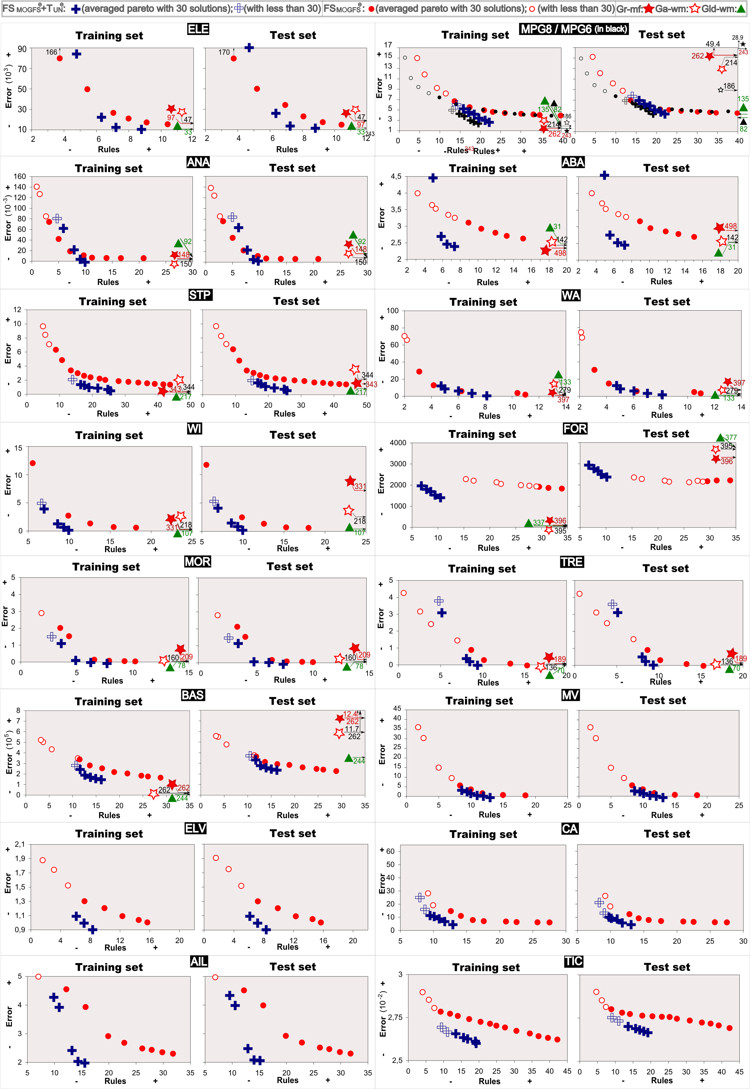
Figure 1. Average Pareto fronts obtained by FSMOGFSe, FSMOGFSe+TUNe and average solutions obtained by GR-MF, GA-WM and GLD-WM on the different data sets.

Complementary Material 2:

Some examples on the influence of the Lateral Displacements and the Rule Cropping Strategy

This section briefly analyzes the influence of the lateral displacements and the rule cropping strategy in the proposed method. In order to better analyze the learning method performance, two versions of FSMOGFS (without fast error estimation) have been adapted by avoiding both components separately in order to compare with the original version. In this way, some results have been obtained by considering some representative data sets selected as particular examples of non desirable effects.

On the lateral displacements: To analyze the influence of the lateral displacements we modified FSMOGFS by keeping α values equal to zero, by only using the integer part of the chromosome and by applying the incest prevention on this part. The results obtained by this new version are shown and compared with the original version in Table 2 on ELE and ABA data sets. Additionally, we have also considered the two most complex problems, AIL and TIC, as examples on high dimensional datasets and in order to also show the effects in the post-processing stage. The values in these kinds of tables are the same explained for Table 1. In ELE, the effect of avoiding the lateral displacements is an important lost of accuracy in both training and test. However, it is not the only effect that can be detected by taking into account the ABA data set. In this case, the algorithm was unable to find promising simpler partitions as in the case of using the α parameters (the number of rules becomes higher). The reason is that those simpler partitions seems not good in their initial positions and the algorithm is not able to detect them as promising, then choosing more complex partitions that represent a better accuracy. This is the opposite in the case of AIL and TIC. The algorithm is focussing on too simple partitions, which are not the most appropriate for a further fine parameter tuning. Even though that the post-processing stage will be able to partially alleviate the effects of not using lateral displacements in some cases, by taking into account the results obtained for AIL and TIC we can see that it significantly affects in others. A smaller number of rules with a bad performance were finally obtained for AIL and much more rules with not better results were obtained for TIC after the post-processing stage as a consequence of not using the small lateral displacements in the first learning stage.

In this way, the use of the α parameters can be considered as a screening on the granularity configuration that allows the detection of promising partitions in a closed zone around their initial positions.

Table 2. Influence of the lateral parameters in four example data sets: ELE and ABA (first stage effects); AIL and TIC (first and second stage effects)

Version	#R/V	Tra.	SD Tra	Tst.	SD Tst	Version	R/V	Tra.	SD Tra	Tst.	SD Tst
ELE: Size 1056, 4 variables						ABA: Size 4177, 8 variables
FSMOGFS	10/2	16018	314	16083	1108	FSMOGFS	17/3	2.682	0.149	2.697	0.204
α: 0.0	10/2	20611	433	20614	1379	α: 0.0	23/4	2.817	0.127	2.848	0.222
AIL: Size 13750, 40 variables
FSMOGFS	33/4	2.305	0.21	2.308	0.206	FSMOGFS + TUN	20/4	1.864	0.221	1.905	0.233
α: 0.0	28/4	3.010	0.156	3.052	0.160	α: 0.0 + TUN	13/4	2.631	0.034	2.678	0.079
TIC: Size 5802, 85 variables
FSMOGFS	44/8	0.027	0.000	0.027	0.001	FSMOGFS + TUN	25/7	0.026	0.000	0.027	0.002
α: 0.0	40/7	0.029	0.001	0.029	0.002	α: 0.0 + TUN	39/7	0.028	0.001	0.028	0.001

On the cropping strategy: To analyze the influence of the cropping strategy included in the WM module of FSMOGFS (up to 50 rules only) we modified it by allowing the complete rule generation without limitations and by allowing up to 100 rules. The results obtained by these two versions are shown and compared with the original version in Table 3 on ELE, WIZ and the MPG data sets. In this case, both new versions show an important increment in the number of rules without significant error improvements or even getting worse in two data sets. It is clear that this quantity of rules are not necessary since, even in some cases, the generalization ability of the obtained models decreases at the same time that simplicity is affected. Further, the computational times are also positively affected when the maximum number of rules is 50.

Table 3. Influence of the rule cropping strategy in four example data sets (ELE, WIZ, MPG6 and MPG8)

Version	#R/V	Tra.	SD Tra	Tst.	SD Tst	H:M:S	Version	R/V	Tra.	SD Tra	Tst.	SD Tst	H:M:S
ELE: Size 1056, 4 variables							ABA: Size 4177, 8 variables
FSMOGFS	10/2	16018	314	16083	1108	0:00:08	FSMOGFS	38/3	3.850	0.198	4.820	0.772	0:00:07
#R max: 100	11/2	16131	379	16571	1114	0:00:10	#R max: 100	89/4	3.205	0.194	4.478	0.911	0:00:10
#R max: ∞	11/2	16131	379	16571	1114	0:00:10	#R max: ∞	173/5	2.409	0.150	5.864	1.983	0:00:20
WIZ: Size 1461, 9 variables							MPG8: Size 398, 8 variables
FSMOGFS	23/3	1.469	0.080	1.567	0.223	0:00:35	FSMOGFS	40/3	3.827	0.274	4.453	1.049	0:00:10
#R max: 100	28/3	1.456	0.068	1.571	0.152	0:00:38	#R max: 100	88/5	2.976	0.266	4.489	1.045	0:00:16
#R max: ∞	70/4	1.351	0.061	1.463	0.152	0:01:14	#R max: ∞	204/7	2.021	0.161	6.718	2.400	0:00:33

Highlights: Both, the lateral displacements and the cropping strategy are complementary mechanisms that bias the algorithm to obtain simpler but still accurate solutions avoiding overfitting. Additionally, both help to enhance the convergence and to decrease the computation time required to obtain the final models.

Complementary Material 3:

Some examples on the extracted Knowledge Bases

This section is devoted to show the kinds of models obtained by the proposed algorithm from the point of view of the interpretability. To do this, we depict some representative models in some of the data sets considered in this contribution. In any event, the models obtained by the proposed algorithm at the most accurate solution considering the first fold can be found here for all the datasets used in the paper.

Figure 2 shows one of the most accurate models obtained with FSMOGFS^e, its corresponding refined model by FSMOGFS^e+TUN^e and its counterpart model obtained by GA-WM in ELE. To ease graphic representation, in these figures, the MFs are labeled from l1 to lLⁱ. Nevertheless, such MFs can be associated to a linguistic meaning determined by an expert. In our opinion and by taking into account the small displacements and the uniform distribution of the final MFs obtained by FSMOGFS, if the l1 label of the X3 variable represents "Very small", l1' could be also interpreted as "Very small" as classically has been considered when parameter learning is applied or based on the expert opinion, maintaining the original meaning of such label. This is the case of the model obtained by FSMOGFS^e, and of most of the final MFs obtained by FSMOGFS^e+TUN^e and GA-WM. However, it is clear that the model obtained by GA-WM presents more difficulties to be understood particularly because of the higher number of rules and the higher number of labels.

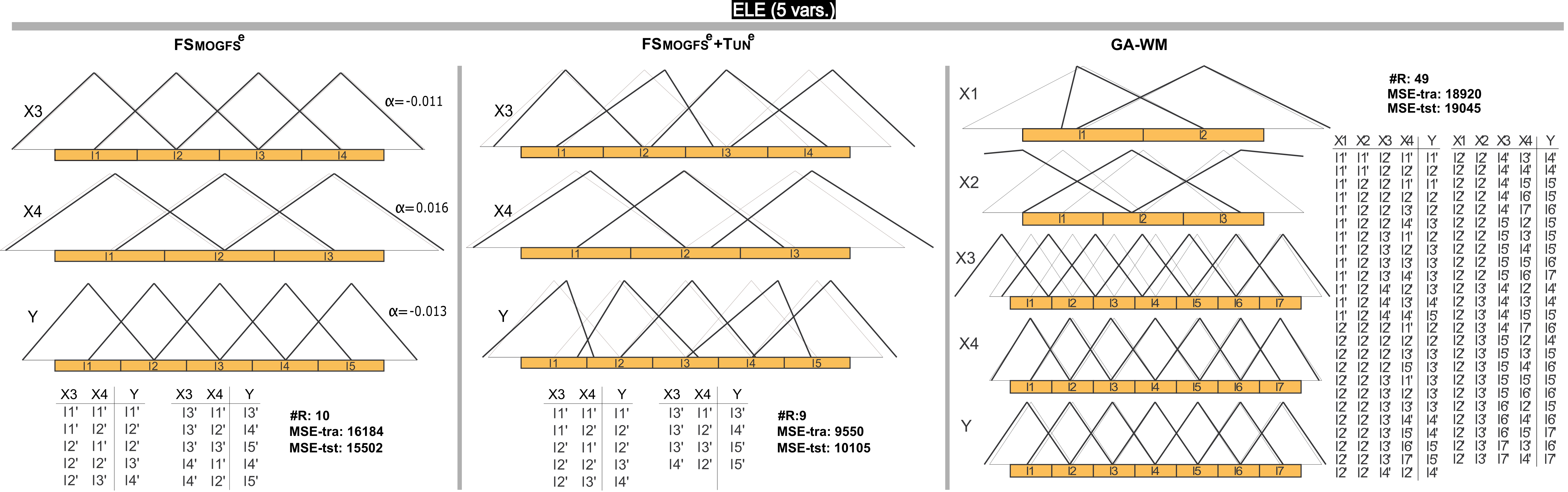
Figure 2. DB with/without learning of parameters (black/gray) and RB of a representative model obtained by FSMOGFSe and FSMOGFSe+TUNe, and their counterpart obtained by GA-WM in the ELE data set

Two of the most interesting data sets considered in this contribution are ELV and AIL due to their complexities. Figure 3 presents two models obtained by FSMOGFSe in these problems. In the first problem, one of the most accurate models obtained from the thirty different runs is shown. It is a very interesting solution with less than a half of the rules obtained in the average results and with very similar training and test errors. It is again an example showing that the error obtained in training can be expected also in test. Besides, this model is a proof on the possibility of obtaining a simple linguistic model in a problem with 18 variables and 16559 cases. On the other hand, the model represented for AIL was selected as an interesting simple model within a Pareto front obtained in the thirty runs. It was selected based on the number of rules and on the training error (which is not so far from the average value of the most accurate solution from each Pareto front obtained in this data set). Again the test error is very similar to the training error. The model is very interesting and descriptive in this high-dimensional problem (40 variables), representing a very good alternative depending on the user necessity. Since FSMOGFSe+TUNe is applied in two stages, these kinds of simple models also represents a possibility to apply the second stage in order to obtain very accurate but actually highly simple models.

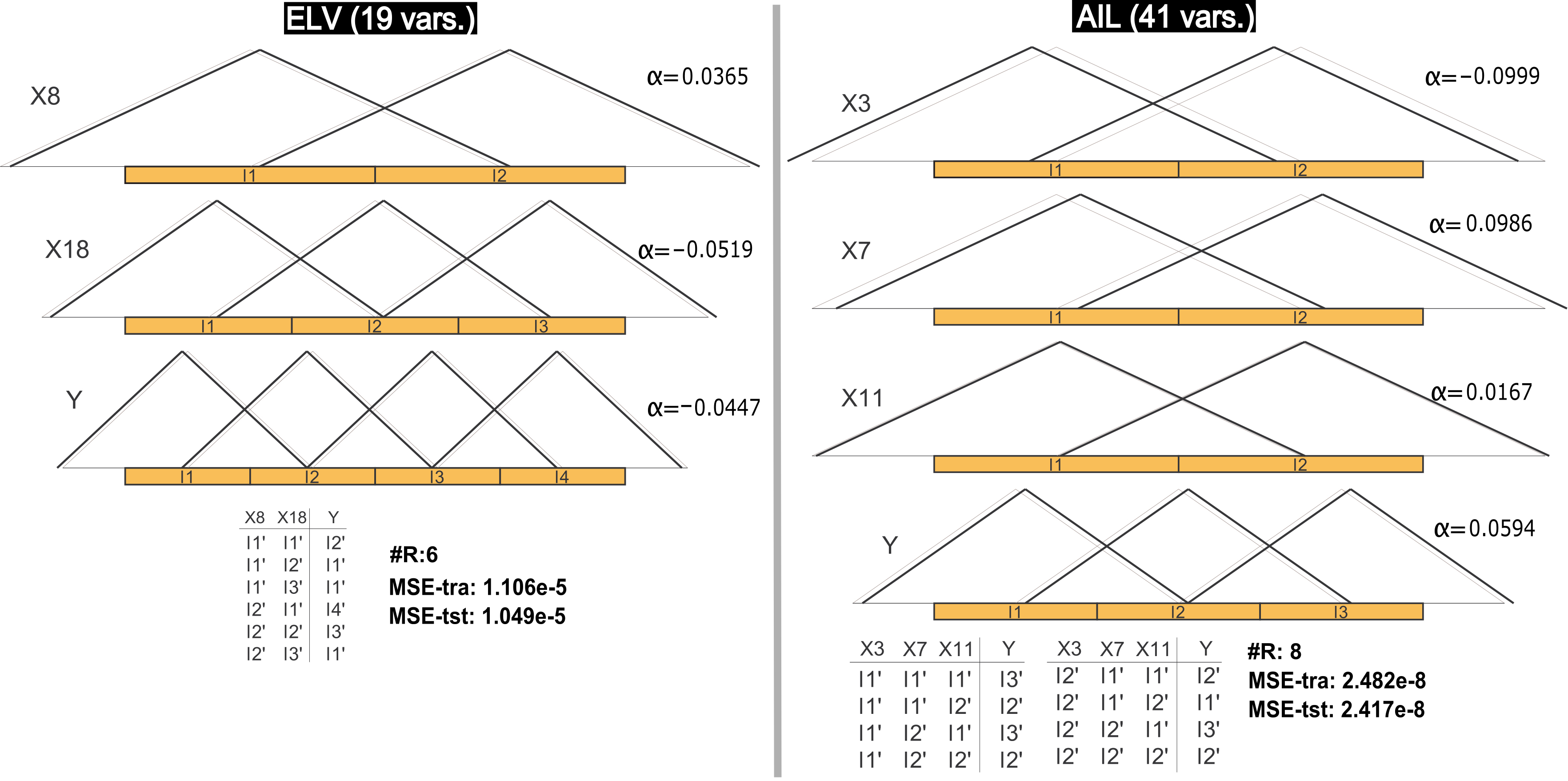
Figure 3. DB with/without learning of parameters (black/gray) and RB of a representative model obtained by FSMOGFSe in the ELV and AIL data sets

Complementary Material 4:

Tables of results and tables with Wilcoxon's Signed Rank test for two different running conditions of the comparison methods, GR-MF, GA-WM and GLD-WM (number of labels in {2,...,7} or {3,...,9}). Results , Wilcoxon

 

 

 

Summary: Here we include complementary material in order to show the results obtained by the comparison methods, GR-MF, GA-WM and GLD-WM, in two different running conditions. Taking into account these results, we can select the working mode that obtains the best test errors for these approaches, giving them the possibility of competing in the best conditions.

To this end, we analyze the results of the accuracy oriented single objective based algorithms GR-MF, GA-WM and GLD-WM (O. Cordón, F. Herrera, and P. Villar, "Generating the knowledge base of a fuzzy rule-based system by the genetic learning of the data base," IEEE Transactions on Fuzzy Systems, vol. 9, no. 4, pp. 667-674, 2001, O. Cordón, F. Herrera, L. Magdalena, and P. Villar, "A genetic learning process for the scaling factors, granularity and contexts of the fuzzy rule-based system data base," Information Sciences, vol. 136, pp. 85-107, 2001 and R. Alcalá, J. Alcalá-Fdez, F. Herrera and J. Otero, "Genetic Learning of Accurate and Compact Fuzzy Rule Based Systems Based on the 2-Tuples Linguistic Representation". International Journal of Approximate Reasoning vol. 44:1, pp. 45-64, 2007 respectively) with the granularity configuration indicated by the authors in their original papers ({3,...,9}) and with the one used by the algorithm proposed in the contribution under submission ({2,...,7}). Taking into account these results (see Table 4 or download it here), we can select the working mode that obtains the best test errors for these approaches, giving them the possibility of competing in the best conditions. In order to assess this decision, we have used Wilcoxon's Signed-Ranks test for pair-wise comparison (a description of Wilcoxon's Signed-Ranks test and an explanation on how to apply it in the regression framework can be found at Complementary Material 5, including a definition of the DIFF column).

The null hypothesis associated with Wilcoxon's test is rejected (p < α) in all the algorithms (but for GLD-WM in Tst.), not only in Tst. but also in the number of rules, in favour of versions in {2,...,7} due to the differences between R⁺ and R^- (see the corresponding Table here). In any event, the version in {2,...,7} for GLD-WM obtains better rankings in Tst.

These tables, results and Wilcoxon's assessment, can be also downloaded as an Excel document by clicking on the following links, and respectively.

Table 4. Average results of GR-MF, GA-WM and GLD-WM (Rules/Training/Test) by allowing granularities in {3,..., 9} and {2,..., 7}. Results in this table (Tra./Tst.) should be multiplied by $10^5$ in the case of Bas.

Data set	GR-MF(3-9)			GR-MF(2-7)						GA-WM(3-9)			GA-WM(2-7)						GLD-WM(3-9)			GLD-WM(2-7)
NAME(V/Size)	R	Tra	Tst	R	Tra	Tst	DIFFTst	DIFFR		R	Tra	Tst	R	Tra	Tst	DIFFTst	DIFFR		R	Tra	Tst	R	Tra	Tst	DIFFTst	DIFFR
Ele(4/1056)	96	16374	18067	97	16645	18637	-0.032	-0.010		73	13274	15054	47	17230	18977	-0.261	0.356		41	9750	11738	33	11483	13384	-0.140	0.195
Mpg6(5/398)	242	1.451	28.164	243	1.423	28.933	-0.027	-0.004		246	1.165	28.232	186	1.879	8.824	0.687	0.244		189	1.269	5.182	82	2.294	4.387	0.153	0.566
Mpg8(7/398)	261	1.371	54.802	262	1.356	49.360	0.099	-0.004		259	0.947	44.800	214	1.563	15.216	0.660	0.174		216	1.027	4.847	135	1.709	4.782	0.013	0.375
Ana(7/4052)	208	0.004	0.021	148	0.005	0.017	0.190	0.288		196	0.002	0.016	150	0.003	0.008	0.500	0.235		121	0.003	0.005	92	0.006	0.008	-0.559	0.240
Aba(8/4177)	496	2.365	2.855	498	2.358	2.885	-0.011	-0.004		300	2.279	2.586	143	2.433	2.549	0.014	0.523		58	2.373	2.481	31	2.487	2.545	-0.026	0.466
Stp(9/950)	458	0.292	5.674	343	0.400	1.543	0.728	0.251		449	0.278	2.587	344	0.389	2.192	0.153	0.234		311	0.223	0.373	217	0.299	0.435	-0.166	0.302
Wiz(9/1461)	537	0.871	19.602	331	1.176	9.602	0.510	0.384		361	0.963	10.757	218	1.233	3.529	0.672	0.396		212	0.794	1.231	107	0.926	1.150	0.065	0.495
Wan(9/1609)	602	1.159	12.882	397	1.406	7.381	0.427	0.341		436	1.219	5.136	279	1.522	2.820	0.451	0.360		295	1.034	1.689	133	1.111	2.075	-0.228	0.549
For(12/517)	402	95	2440	396	113	3300	-0.352	0.015		402	21	2445	395	47	3693	-0.510	0.017		393	30	4911	377	49	3847	0.217	0.041
Mor(15/1049)	260	0.029	0.308	209	0.030	0.176	0.429	0.196		224	0.017	0.176	160	0.020	0.093	0.472	0.286		127	0.013	0.024	78	0.016	0.022	0.064	0.386
Tre(15/1049)	255	0.048	0.169	189	0.066	0.144	0.148	0.259		220	0.039	0.101	136	0.045	0.064	0.366	0.382		139	0.032	0.049	70	0.033	0.045	0.065	0.496
Bas(16/337)	266	0.153	14.077	262	0.255	12.439	0.116	0.015		264	0.128	13.184	262	0.202	11.706	0.112	0.008		253	0.084	3.688	244	0.138	3.610	0.021	0.036

Complementary Material 5:

Wilcoxon's Signed-Ranks test and its application in the regression framework

A non-parametric test is that which uses nominal data or ordinal data or data represented in an ordinal way of ranking. This does not imply that only they must be used for these types of data. It could be very interesting to transform the data from real values contained within an interval to ranking based data, in the same way that a non-parametric test can be applied over typical data of a parametric test when they do not fulfill the necessary conditions imposed by the use of the test. In the following, we explain how the Wilcoxon's Signed-Ranks test can be applied to the regression framework and we present the basic functionality of this non-parametric test for pair-wise comparisons.

Application of Wilcoxon's test in the regression framework: Wilcoxon's test is based on computing the differences between two sample means (typically, mean test errors obtained by a pair of different algorithms on different datasets). In the classification framework these differences are well defined since these errors are in the same domain. In our case, to have well defined differences in the MSE or in the number of rules, we propose to adopt a normalised difference DIFF, defined as:

$$DIFF=\frac{MEan(Other)-Mean(NewApproach)}{Mean(Other)}$$

where Mean(x) represents the means obtained by the x algorithm on the MSE or the number of rules. This difference expresses the improvement rate of a new algorithm or approach. Positive values indicate an improvement for the new algorithm while negative represents a worst performance. Rankings are computed by considering the absolute value of DIFF for the winner algorithm and zero for the other in each data-set.

Wilcoxon's signed-rank test: The Wilcoxon signed-rank test is a pair-wise test with the aim of detecting significant differences between two sample means: it is analogous to the paired t-test in non-parametric statistical procedures. If these means refer to the outputs of two algorithms, then the test practically assesses the reciprocal behavior of the two algorithms (D. Sheskin, Handbook of parametric and nonparametric statistical procedures. Chapman & Hall/CRC, 2003 and F. Wilcoxon, "Individual comparisons by ranking methods," Biometrics, vol. 1, pp. 80–83, 1945).

Let d_i be the difference between the performance scores of the two algorithms on the i-th out of N_ds data-sets. The differences are ranked according to their absolute values; average ranks are assigned in case of ties. Let R⁺ be the sum of ranks for the datasets on which the first algorithm outperformed the second, and R^- the sum of ranks for the contrary outcome. Ranks of d_i = 0 are split evenly among the sums; if there is an odd number of them, one is ignored:

$$R^+=\displaystyle\sum_{d_i>0}rank(d_i)+\frac{1}{2}\displaystyle\sum_{d_i=0}rank(d_i), R^-=\displaystyle\sum_{d_i<0}rank(d_i)+\frac{1}{2}\displaystyle\sum_{d_i=>0}rank(d_i)$$

Let T be the smaller of the sums, T = min(R⁺,R^-). If T is less than, or equal to, the value of the distribution of Wilcoxon for N_ds degrees of freedom (Table B.12 in J. Zar, Biostatistical Analysis. Upper Saddle River, NJ: Prentice-Hall, 1999), the null hypothesis of equality of means is rejected.

Complementary Material 6:

Lateral Tuning of Membership Functions

In (R. Alcalá, J. Alcalá-Fdez, and F. Herrera , A proposal for the genetic lateral tuning of linguistic fuzzy systems and its interaction with rule selection, IEEE Trans. Fuzzy Syst., vol. 15, no. 4, pp. 616–635, 2007), a new model of tuning of FRBSs was proposed considering the linguistic 2-tuples representation scheme introduced in (F. Herrera and L. Martínez , A 2-tuple fuzzy linguistic representation model for computing with words, IEEE Trans. Fuzzy Syst., vol. 8, no. 6, pp. 746–752, 2000), which allows the lateral displacement of the support of a label and maintains the interpretability at a good level. This proposal introduces a new model for rule representation based on the concept of symbolic translation. The symbolic translation of a label is a number in [-0.5, 0.5). This interval defines the variation domain of a label when it is moving between its two adjacent lateral labels, i.e., it represents the range to determine the relative shifts associated to the labels (see Figure 4a). Let us consider a generic linguistic fuzzy partition S = { s₁, ..., s_L } (with L representing the number of labels). Formally, we represent the symbolic translation of a label s_iin S by means of the 2-tuple notation,

The symbolic translation of a label involves the lateral displacement of its associated MF. Figure 4 shows the symbolic translation of a label represented by the 2-tuple (s₂, -0.3) together with the associated lateral displacement of the corresponding MF. Both the linguistic 2-tuples representation model and the elements needed for linguistic information comparison and aggregation, were presented and applied to the Decision Making framework.

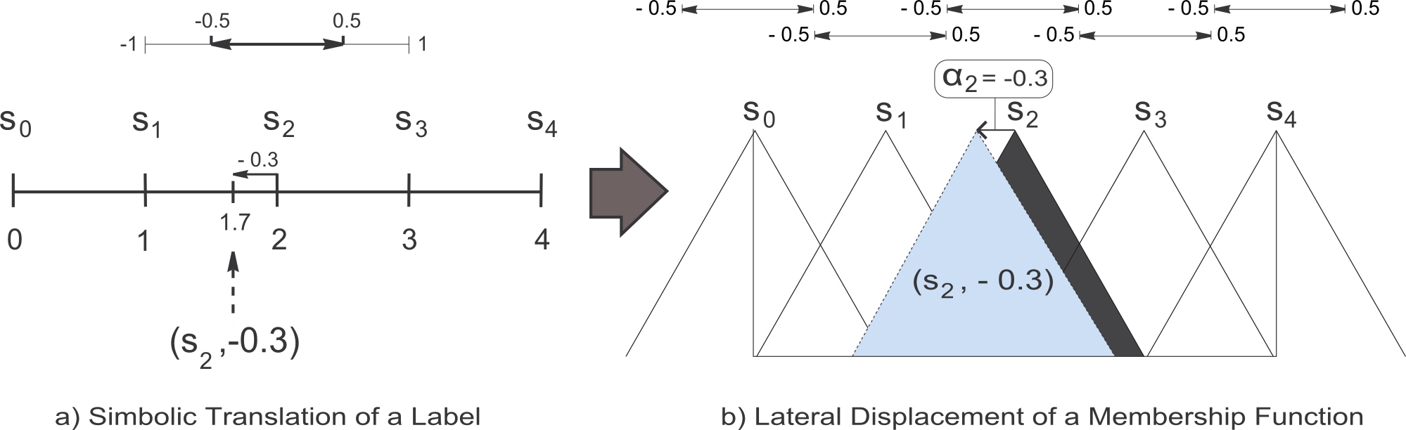
Figure 4. Symbolic translation of the linguistic label s2 considering the set of labels S = { s0, s1, s2, s3, s4}

In the context of FRBSs, the linguistic 2-tuples could be used to represent the MFs comprising the linguistic rules. This way to work, introduces a new model for rule representation that allows the tuning of the MFs by learning their respective lateral displacements. The main achievement is that, since the 3 parameters usually considered per label are reduced to only 1 symbolic translation parameter, this proposal decreases the learning problem complexity easing indeed the derivation of optimal models. Other important issue is that, the learning of the displacement parameters keeps the original shape of the MFs (in our case triangular and symmetrical). In this way, from the parameters α applied to each label, we could obtain the corresponding triangular MFs, by which a FRBS based on linguistic 2-tuples could be represented as a classical Mamdani FRBS.