This Website contains two complementary documents related to the paper under submission:

J. Luengo, F. Herrera , An Automatic Extraction Method of the Domains of Competence for Learning Classifiers using Data Complexity Measures.

Summary:

1. Paper abstract
2. Description of the Fuzzy Rule Based Classification methods
3. Data sets generation
4. Tables with the accuracy results for the different classification methods used in the paper
5. Automatic method software

Paper abstract

The constant appearance of algorithms and problems in Data Mining make impossible to know in in advance whether the model will perform well or poorly until it is applied, which can be costly. It would be useful to have a procedure which indicates, prior to the application of the learning algorithm and without needing a comparison with other methods, if the outcome will be good or bad using the information available in the data.

Using a set of data complexity measures proposed for the task of classification, in this work we present an automatic extraction method to determine the domains of competence of a classifier. These domains codify the characteristics of the problems that are suitable or not for it, relating the concepts of data geometrical structures that may be difficult and the final accuracy obtained by any classifier. In order to do so, this proposal uses twelve metrics of data complexity acting over a large benchmark of data sets in order to analyze the behavior patterns of the method, obtaining intervals of data complexity measures with good or bad performance. As a representative classifiers to analyze the proposal, three classical but different algorithms are used: C4.5, SVM and K-NN.

From these intervals two simple rules that describe the good or bad behaviors of the classifiers mentioned each are obtained, allowing the user to characterize the response quality of the methods from the data set complexity metrics of a given data set. These two rules have been validated using fresh problems, showing that they are general and accurate. Thus, it can be established when the classifier will perform well or poorly prior to its application.

Description of the automatic extraction method

Summary: In this section we provide the algorithmic description of the automatic extraction method used in the associated paper. This description is extendend, as all the algorithm mentioned in the paper are considered and presented here. The notation used is the same as the paper one. Next we include here the same initial definitions given in the paper for the sake of completeness.

 

The automatic extraction method analyzes a list of data sets where each complete data set has an associated performance measure of the classifier considered (typically the training and test accuracy rates) and the values of the twelve Data Complexity Measures (DCMs).

Definition 1 Let U={u₁,u₂,...,u_n} be a list of n different data sets. Each data set u_i has associated a tuple T_ui=(u_i^tra, u_i^tst, u_i^F1, u_i^F2,…,u_i^T2) where u_i^tra is the training accuracy value associated with the data set u_i for a specific classifier, u_i^tst is the test accuracy value associated with the data set u_i for the same classifier, and the set CM_ui = {u_i^F1, u_i^F2,…,u_i^T2} contains the values for the twelve DCMs.

Definition 2 Given a list of data sets U={u₁,u₂,...,u_n}, we define the average training accuracy over U as ―U^tra = [1/n] ∑_i=1ⁿ u_i^tra and the average test accuracy as ―U^tst = [1/n] ∑_i=1ⁿ u_i^tst.

In order to define the domains of competence of an classifier, intervals of values of the DCMs need to be stated. The intervals are defined over the list U of data sets, sorting the list U by one DCM CM_j of the twelve DCMs represented in the T tuple, defined as follows.

Definition 3 A sorted list of data sets U_CMj with respect to the data complexity CM_j is such that ∀u_i^CM_j,u_j^CM_j ∈ U_CMj; u_i^CM_j ≤ u_j^CM_j, if i < j.

Definition 4 Given a list of sorted data sets U_CMj={u₁,u₂,...,u_n} by the DCM CM_j ∈ T, we consider an interval V = {u_i,u_i+1,…,u_l} ⊆ U_CMj where the lower and upper bound values of V immediately follows:

1. M_low(V) = min_k {u_k^CM_j ∈ V} = u_i.
2. M_up(V) = max_k {u_k^CM_j ∈ V} = u_l.

The domains of competence are set based on a range of a DCM values. The automatic extraction method first tries to find a point of outstanding performance for the classifier (vary good or very bad). Using such a point as a seed, it tries to add contiguous points (i.e. data sets with training and test values) to it, in order to conform an interval.

Good and bad behavior elements

The distinction between good and bad behavior elements is based upon the absence or presence of overfitting, respectively, as well as the test accuracy value obtained. These are the two most common elements to determine when a classification algorithm performs well or poorly. The automatic method works with specific values, depending on the data sets which act as a sample of the classifier’s behavior, so we need to parameterize these two subjective indicators.

The former aspect is evaluated comparing the element’s difference between training and test accuracy with respect to the global average. This global average difference is straightforwardly defined as

$$U^{diff}=\frac{1}{n} \displaystyle\sum_{j=1}^{n}u_j^{tra}-u_j^{tst}$$ (1)

An element with a difference between training and test accuracy above this average is considered to be overfitted, while the opposite case is not.

On the other hand any good behavior element u_i must present a minimum test accuracy value u^test_i , represented by the minGoodElementTest. By contrast a bad behavior element u_j shows a test accuracy value u^test_i under the same threshold minGoodElementTest.

Definition 5 A good behavior element u_i is such that

1. u_i^test ≥ minGoodElementTest; and
2. u_i^tra − u_i^tst ≤ [1/n] ∑_j=1ⁿ u_j^tra−u_j^tst.

Definition 6 A bad behavior element u_i is such that

• u_i^test < minGoodElementTest; and
• u_i^tra − u_i^tst > [1/n] ∑_j=1ⁿ u_j^tra−u_j^tst.

Good and bad behavior intervals

The good or bad behavior intervals V shows the good or bad performance of the classifier over a range of elements on average. Thus, for intervals, the definition of good or bad behavior is different with respect to individual elements, although they share the same underlying concepts: overfitting and test accuracy.

We consider the average difference across every element covered as a criteria to discriminate between good and bad behavior. The average interval V difference is defined as

$$V^{diff}=\frac{1}{|V|} \displaystyle\sum_{u_j \in V}^{n}u_j^{tra}-u_j^{tst}$$ (2)

A good interval must have a lower average difference than the global average ̅U_diff defined in Equation (1). A bad interval must verify the opposite case.

We also establish a threshold between the average test accuracy of the interval ―V^tst and the global average ―U^tst. An interval of good behavior must have an average test accuracy above this threshold plus ―U^tst, while a bad behavior interval must verify the opposite case: ―U^tst minus the threshold. This condition reflects the behavior difference of the classifier with respect to the average obtained in the data set sample.

In the case of good behavior intervals, we also establish that no element can have a test accuracy below minGoodIntervalTest percent. The reason to do so is to avoid very bad elements being covered by the interval due to the latter still having a good test average. This aspect is not crucial when defining bad intervals.

Definition 7 An interval of good behavior V = {u_i,…,u_j} is such that

1. ―V^diff ≤ ―U^diff; and
2. ―V^tst ≥ ―U^tst + threshold; and
3. ∀u_j ∈ V; u_j^tst ≥ minGoodIntervalTest

Definition 8 An interval of bad behavior V = {u_i,…,u_j} is such that

• ―V^diff > ―U^diff; and
• ―U^tst < ―U^tst − threshold.

Automatic extraction method description

The automatic extraction method obtains a series of good or bad behavior intervals (as indicated in Definitions 7 and 8 respectively) from a list of data sets U. Each data set u_i ∈ U has the associated tuple T containing the training and test accuracy values for a particular classifier (C4.5, SVM or K-NN in this case) and its twelve data complexity values.

In order to extract the good and bad behavior intervals, the automatic extraction method arranges the data sets in U by sorting them with one of the DCMs CM_j, j=1,…,12, obtaining a new sorted list U_CMj. Then the sorted list U_CMj is explored from the lowest to highest values of CM_j. When a good or bad behavior element u_i ∈ U_CMj is found (Definitions 5 and 6 respectively), the exploration stops. The found element u_i is considered as an initial interval V={u_i}, which is extended by adding the adjacent elements to u_i. This growing process continues while the interval V verifies the definitions of good or bad behavior intervals accordingly. A final interval V={u_i−r,…,u_i,…,u_i+s}; r,s ∈ \mathbbN is obtained when the corresponding definition is not met.

When all the possible intervals have been extracted, a final cleaning process is applied, in order to merge overlapped or slightly separated intervals of the same type, provided that the corresponding definition of a good or bad interval is maintained. Finally, a filtering is applied in order to avoid non-significant intervals where intervals with a support under 15% of the total data sets are discarded.

We present the main outline of the automatic extraction method described in Algorithm 1.

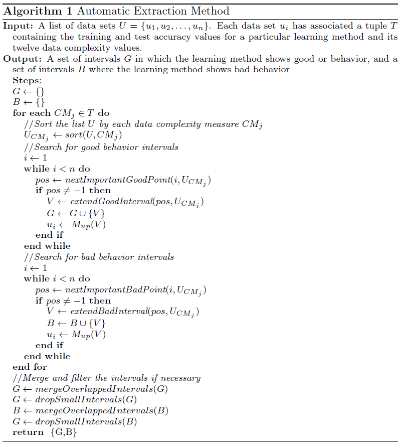
Main outline of the automatic extraction method

The functions used in the algorithm are described as follows:

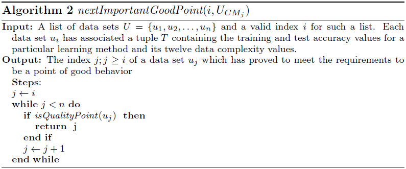
• nextImportantGoodPoint(i, U): Looks for the index k of the next good behavior point u_k in the subset V = {u_i,…,u_n} ⊆ U. If no good behavior point can be found it returns −1.

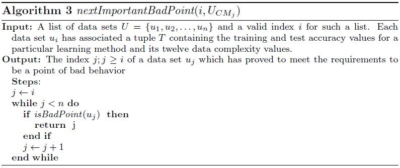
• nextImportantBadPoint(u_i, U): Looks for the index k of the next bad behavior point u_k in the subset V = {u_i,…,u_n} ⊆ U. If no bad behavior point can be found it returns −1.

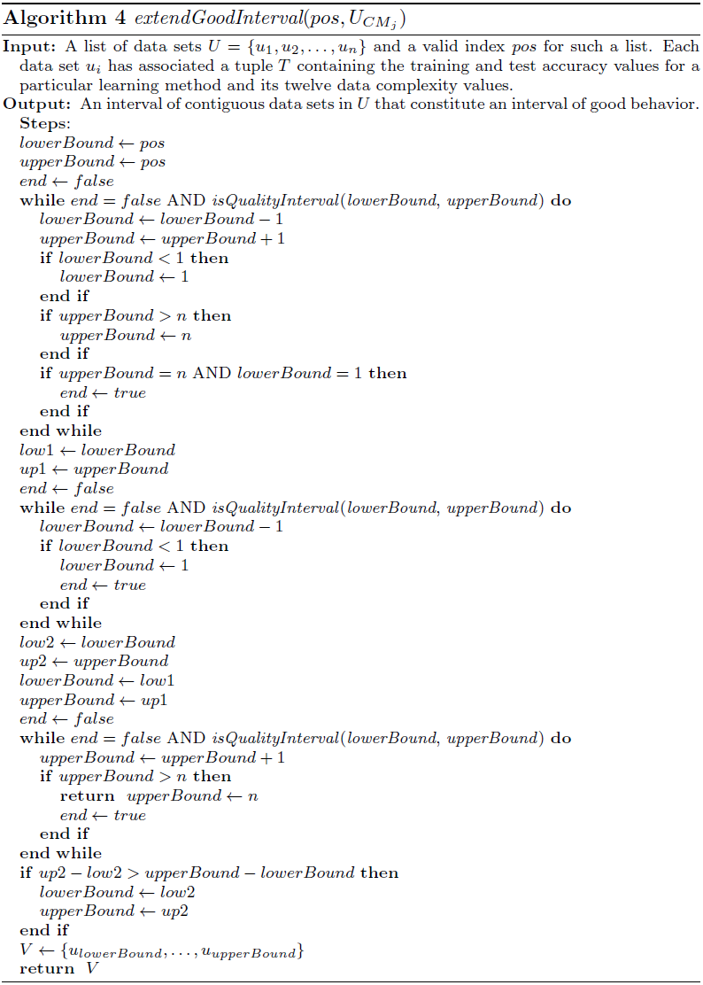
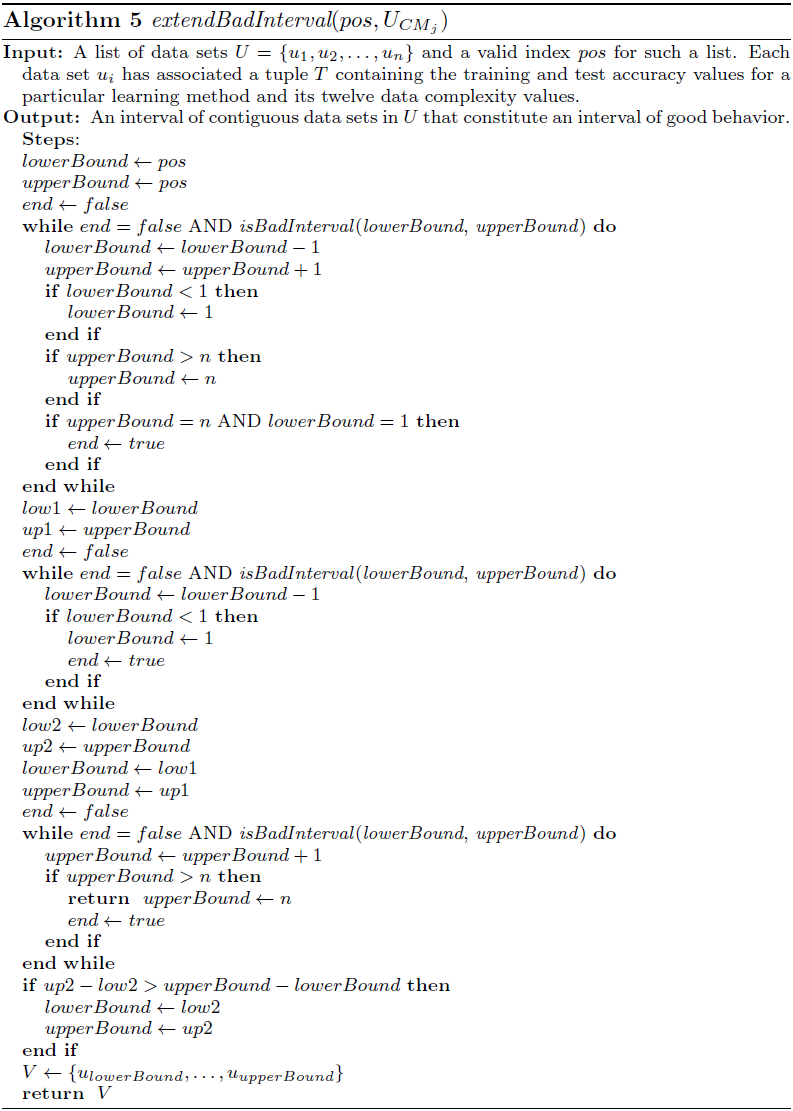
• extendGoodInterval(pos,U): From the reference point u_pos this method creates a new interval of good behavior V = {u_pos−r,…,u_pos,…,u_pos+s} ⊆ U, maintaining the element's order in U.

• extendBadInterval(pos,U): From the reference point u_pos this method creates a new interval of bad behavior V = {u_pos−r,…,u_pos,…,u_pos+s} ⊆ U, maintaining the element's order in U.

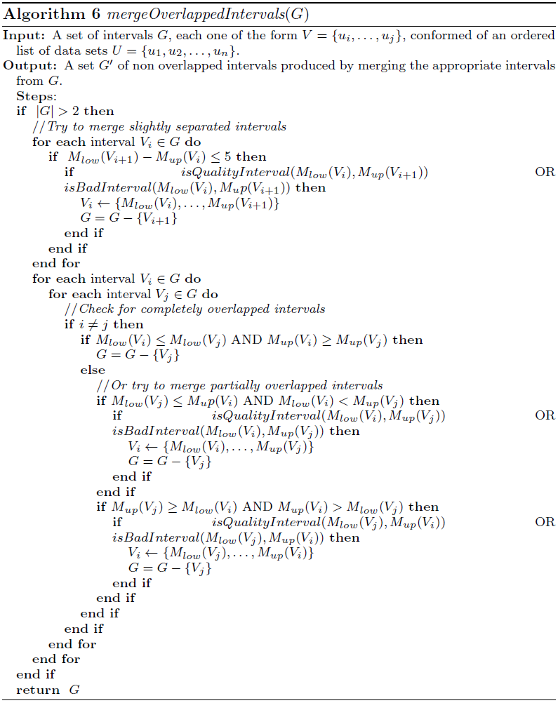
• mergeOverlappedIntervals(A): In this function, an interval V_k is dropped from A if ∃V_m ∈ A; M_up(V_m) ≥ M_up(V_k) and M_low(V_m) ≤ M_low(V_k). Moreover it tries to merge overlapped intervals V_k, V_m; V_k ∩V_m ≠ ∅; or intervals separated by a maximum gap of 5 elements (data sets), provided that the new merged intervals satisfy Definition 7 and 8 of good or bad behavior respectively.

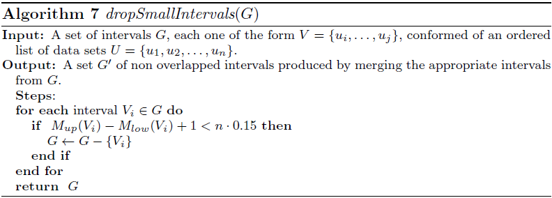
• dropSmallIntervals(A): This function discards the intervals V_k ∈ A which contains a number of data sets less than 15% ·n.

Data sets generation

In this paper a set of binary classification problems have been used. Initially, these problems were generated from pairwise combinations of the classes of 26 problems from the Keel Dataset Repository. The ones selected were abalone, australian, balance, bupa, cars, contraceptive, ecoli, solar-flare, glass, hayes-roth, iris, kr vs. k, led7digit, mammographic, marketing, monks, new-thyroid, optdigits, penbased, segment, tae, texture, vowel, wine, yeastB and zoo.

In order to do this, first we take each data set and extract the examples belonging to each class. Then we construct a new data set with the combination of the examples from two different classes. This will result in a new data set with only 2 classes and the examples which have two such classes as output. For example, one data set obtained from iris with this procedure could contain only the examples of Iris-setosa and Iris-virginica and not those from Iris-versicolor.

This method for generating binary data sets is limited by the combinatoric itself, and we can only obtain over 200 new data sets with the original 21 data sets with this first approach. In order to obtain additional data sets we group the classes two by two, that is, we create a new binary data set, and each of its two classes are the combination of two original classes. For this second approach we have used ecoli, glass, and shuttle data sets, since they have a high number of class labels. For example, using ecoli we can create a new binary data set combining cp and im classes into a new one (say class “A“), and pp and imU (say new class “B”). The new data set would contain only the examples of classes cp, im, pp and imU, but their class label now would be “A“ if their original class was cp or im, and “B” if it was pp or imU.

It is important to note that not all the data sets generated by this procedure may be valid. In order to avoid the data sets that may yield erroneous conclusions, we filter those created data sets that resulted to be too easy for the classification task, or present an imbalanced ration between the classes. If the data set proves to be linearly-separable, then we may classify it with a linear classifier with no error and such a data set would not be a representative problem. The complexity measure L1 indicates if a problem is linearly-separable when its value is zero, so every data set with an L1 value of zero is discarded. On the other hand, we limit the imbalance ratio to a value of 1.5, as it has been analyzed in the literature as a reasonable threshold to denote balanced data sets that enable the use of accuracy as a performance measure (as used by the DCMs as well). This filtering resulted in 295 binary classification problems which are used as our training-bed for the automatic extraction method.

In order to validate the results obtained in our analysis, we have applied the same methodology to the yeast, flare, car, letter, segment, marketingand texture data sets from the KEEL Dataset repository, due to their high number of classes. Applying the same filtering criteria, we have obtained another 1428 data sets used for validating the rules obtained in our analysis which provide enough values for each data complexity measure to be representative.

Tables with the accuracy results for the different classification methods used in the paper

Summary: In this section we present the accuracy results obtained for each classification method. These are the complete results from the study performed. Both training and test accuracy are present for each classifier.

We have used a 10-fcv validation scheme. We have calculated the 12 data complexity measures for each data set.

These tables can be downloaded as an Excel document by clicking on the following links:

1. C4.5 accuracy results for the obtention of its domains of competence with the initial 295 data sets and the intervals obtained by the automatic extraction method .
2. SVM accuracy results for the obtention of its domains of competence with the initial 295 data sets and the intervals obtained by the automatic extraction method .
3. K-NN accuracy results for the obtention of its domains of competence with the initial 295 data sets and the intervals obtained by the automatic extraction method .

Using the intervals obtained it is possible to generate the collective rules as described in the paper (see the next section Automatic method software in order to do so). Such collective rules are contained in the following Excel files, also providing the graphical representation as depicted in the associated paper:

1. C4.5 collective rules and the three regions of competence: good, bad and not characterized .
2. SVM collective rules and the three regions of competence: good, bad and not characterized .
3. K-NN collective rules and the three regions of competence: good, bad and not characterized .

Once the collective PRD and NRD-PRD rules have been extracted, the fresh extra bunch of 1428 data sets are used in order to validate the domains of competence defined by such rules. The distribution of the data sets among the rules is contained in the following Excel files, also providing the graphical representation as depicted in the associated paper:

1. C4.5 validation results and the three regions of competence: good, bad and not characterized .
2. SVM validation results and the three regions of competence: good, bad and not characterized .
3. K-NN validation results and the three regions of competence: good, bad and not characterized .

Automatic extraction method software

Summary: In this section we provide the automatic method source code written in JAVA. It has been developed using the Netbeans IDE so it is possible to use it to further develope the code. The source code has been licensed using the GPLv3.

The program is written in JAVA 6, so an installed JVM in the computer is needed in order to run it.

Obtaining the domains of competence

There are two ways to run the program.

The first one needs you to provide a list of text files using the -l option, as well as the threshold and minimun test accuracy value.
java -jar ComplexityRuleExtraction.jar -l < data file > -h < threshold > -m < minimumTestValue >
This mode will generate a similar output to the previous case, but using all the data complexity measures provided.

The second and last option uses a single text file with all the data complexity measures in a tabbed manner with the -t option.
java -jar ComplexityRuleExtraction.jar -t < data file > -h < threshold > -m < minimumTestValue >

An example of data to be used with the -t option can be found here . Each row in the text file represents one single datasets, where the first column is its name, followed by the 12 data complexity measure values and finally the training and test accuracy values obtained for a single classifier. Please note that the data complexity measures order is: F1 F2 F3 N1 N2 N3 N4 L1 L2 L3 T1 and T2. It is designed to directly accept data copied and pasted from your favourite calc sheet.

The output is given in tabbed format on standard output so you can copy the results to your favourite spreadsheet program. We recommend to redirect the output to a file in the following manner:
java -jar ComplexityRuleExtraction.jar -t training.txt -h 8 -m 90 > output.txt.

Plotting the intervals obtained using GNUplot

The software is also able to print the intervals graphically. In order to do so, you need to have GNUplot installed in your system. The command 'gnuplot' needs to be in the path as well. You can choose between three output formats when plotting such figures. In order to use any of them, simply add the following options to the command line when running ComplexityRuleExtraction with -t or -l options.

--epscolor prints the intervals found for each data complexity measure in a EPS file in color.
--epsbn prints the intervals found for each data complexity measure in a EPS file in black and white.
--png prints the intervals in color using the PNG format.

Several plotting options can be chosen at once.

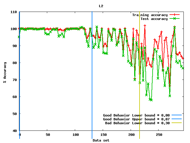
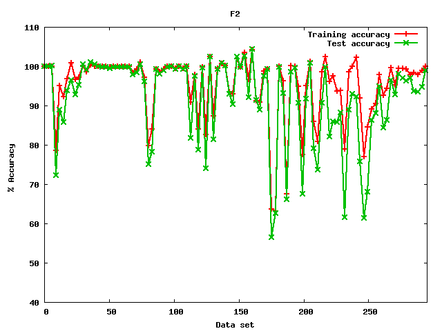
Figure 1: Example of a figure generated by the software where intervals were found	Figure 2: Example of a figure generated by the software where no intervals were found

Summarizing the rules into their disjunctive and conjunctive form

The automatic method also produces two files: good.txt and bad.txt.
These files contains the list of data sets included in the good and bad intervals respectively. They are intended to be used in order to create the conjunction and disjunction of the rules.
We provide a JAR software to carry out this task with no warranty of use which can be downloaded from here . The program should be executed as follows:

java -jar IntersectionConfidence.jar <positive itemset> <negative itemset> <itemset Train and Test text file>
where <positive itemset> corresponds to the good.txt file; and <negative itemset> corresponds to bad.txt. The <itemset Train and Test text file> is a tabbed file with three values per row: the identifier of the data set, the training accuracy and the test accuracy obtained by the classifier. It must contain the same results used to obtain the intervals by the automatic method. An example can be downloaded from here .
It will generate several files:

positiveUnion.txt: It is the union of all the good data sets from good.txt.
negativeUnion.txt: It is the union of all the bad data sets from bad.txt.
intersectionGoodandBad.txt: It is the intersection of the two above unions.
intersectionGoodandNotBad.txt: It is the difference of the union of the good data sets MINUS the union of the bad data sets.
intersectionBadandNotGood.txt: It is the difference of the union of the bad data sets MINUS the union of the good data sets.
remainder.txt: It contains those data sets in <itemset Train and Test text file> not covered by any interval.

How to validate the obtained domains of competence

The software is also capable of reading a previous output with the intervals extracted, and using a new bunch of data sets, it analyzes the covering of such data sets by the rules. Thus the validation of the domains of competence is easily attained. In order to do this, execute:
java -jar ComplexityRuleExtraction.jar -v < intervals file >;< data file > in Windows
java -jar ComplexityRuleExtraction.jar -v < intervals file >:< data file > in Linux

where < intervals file > is the text file with the intervals (i.e. output.txt in the example above) and < data file > refers to a new data file with the same tabbed format as used by the -t option.