Statistical Inference in Computational Intelligence and Data Mining

This Website contains additional material to the SCI2S research group papers on the use of non-parametric tests for data mining and Computational Intellingece:

P1: S. García, F. Herrera, An Extension on "Statistical Comparisons of Classifiers over Multiple Data Sets" for all Pairwise Comparisons. Journal of Machine Learning Research 9 (2008) 2677-2694.
P2: J. Luengo, S. García, F. Herrera, A Study on the Use of Statistical Tests for Experimentation with Neural Networks: Analysis of Parametric Test Conditions and Non-Parametric Tests. Expert Systems with Applications 36 (2009) 7798-7808 doi:10.1016/j.eswa.2008.11.041.
P3: S. García, A. Fernández, J. Luengo, F. Herrera, A Study of Statistical Techniques and Performance Measures for Genetics-Based Machine Learning: Accuracy and Interpretability. Soft Computing 13:10 (2009) 959-977, doi:10.1007/s00500-008-0392-y.
P4: S. García, D. Molina, M. Lozano, F. Herrera, A Study on the Use of Non-Parametric Tests for Analyzing the Evolutionary Algorithms' Behaviour: A Case Study on the CEC'2005 Special Session on Real Parameter Optimization. Journal of Heuristics, 15 (2009) 617-644. doi: 10.1007/s10732-008-9080-4.
P5: S. García, A. Fernández, J. Luengo, F. Herrera, Advanced nonparametric tests for multiple comparisons in the design of experiments in computational intelligence and data mining: Experimental Analysis of Power. Information Sciences 180 (2010) 2044–2064. doi:10.1016/j.ins.2009.12.010.
P6: J. Derrac, S. García, D. Molina, F. Herrera, A Practical Tutorial on the Use of Nonparametric Statistical Tests as a Methodology for Comparing Evolutionary and Swarm Intelligence Algorithms. Swarm and Evolutionary Computation 1:1 (2011) 3-18. doi:10.1016/j.swevo.2011.02.002.
P7: J. Derrac, S. García, S. Hui, P.N. Suganthan, F. Herrera, Analyzing Convergence Performance of Evolutionary Algorithms: A Statistical Approach. Information Sciences 289 (2014) 41-58. doi:10.1016/j.ins.2014.06.009.

The web is organized according to the following summary:

Introduction to Inferential Statistics
Conditions for the safe use of Nonparametric Tests
Nonparametric tests
Case Studies
1. Multiple Comparisons with a control method
2. Multiple Comparisons among all methods
Considerations and Recommendations on the use of Nonparametric tests
1. Considerations on the use of Nonparametric tests
  1. Pairwise Comparisons
  2. Multiple Comparisons with a control method
2. Recommendations on the use of Nonparametric tests
Statistical Analysis of Convergence Performance of Evolutionary Algorithms
Relevant Journal Papers with Data Mining and Computational Intelligence Case Studies
Relevant books on Non-parametric tests
Topic Slides
Software and User's Guide

Introduction to Inferential Statistics

The experimental analysis on the performance of a new method is a crucial and necessary task to carry out in a research on Data Mining, Computational Intelligence techniques. Deciding when an algorithm is better than other one may not be a trivial task.

Hyphotesis testing and p-values: In inferential statistics, sample data are primarily employed in two ways to draw inferences about one or more populations. One of them is the hypothesis testing.

The most basic concept in hypothesis testing is a hypothesis. It can be defined as a prediction about a single population or about the relationship between two or more populations. Hypothesis testing is a procedure in which sample data are employed to evaluate a hypothesis. There is a distinction between research hypothesis and statistical hypothesis. The first is a general statement of what a researcher predicts. In order to evaluate a research hypothesis, it is restated within the framework of two statistical hypotheses. They are the null hypothesis, represented by the notation H0, and the alternative hypothesis, represented by the notation H1.

The null hypothesis is a statement of no effect or no difference. Since the statement of the research hypothesis generally predicts the presence of a difference with respect to whatever is being studied, the null hypothesis will generally be a hypothesis that the researcher expects to be rejected. The alternative hypothesis represents a statistical statement indicating the presence of an effect or a difference. In this case, the researcher generally expects the alternative hypothesis to be supported.

An alternative hypothesis can be nondirectional (two-tailed hypothesis) and directional (one-tailed hypothesis). The first type does not make a prediction in a specific direction; i.e. H1 : µ ≠ 100. The latter implies a choice of one of the following directional alternative hypothesis; i.e. H1:µ > 100 or H1:µ < 100.

Upon collecting the data for a study, the next step in the hypothesis testing procedure is to evaluate the data through use of the appropriate inferential statistical test. An inferential statistical test yields a test statistic. The latter value is interpreted by employing special tables that contain information with regard to the expected distribution of the test statistic. Such tables contain extreme values of the test statistic (referred to as critical values) that are highly unlikely to occur if the null hypothesis is true. Such tables allow a researcher to determine whether or not the results of a study is statistically significant.

The conventional hypothesis testing model employed in inferential statistics assumes that prior to conducting a study, a researcher stipulates whether a directional or nondirectional alternative hypothesis is employed, as well as at what level of significance is represented the null hypothesis to be evaluated. The probability value which identifies the level of significance is represented by α.

When one employs the term significance in the context of scientific research, it is instructive to make a distinction between statistical significance and practical significance. Statistical significance only implies that the outcome of a study is highly unlikely to have occurred as a result of chance, but it does no necessarily suggest that any difference or effect detected in a set of data is of any practical value. For example, no-one would normally care if algorithm A in continuos optimization solves the sphere function to within 10-10 of error of the global optimum and algorithm B solves it within 10-15. Between them, statistical significance could be found, but in practical sense, this difference is not significant.

Instead of stipulating a priori a level of significance α, one could calculate the smallest level of significance that results in the rejection of the null hypothesis. This is the definition of p-value, which is an useful and interesting datum for many consumers of statistical analysis. A p-value provides information about whether a statistical hypothesis test is significant or not, and it also indicates something about “how significant” the result is: The smaller the p-value, the stronger the evidence against the null hypothesis. Most important, it does this without committing to a particular level of significance.

The most common way for obtaining the p-value associated to a hypothesis is by means of normal approximations, that is, once computed the statistic associated to a statistical test or procedure, we can use a specific expression or algorithm for obtaining a z value, which corresponds to a normal distribution statistics. Then, by using normal distribution tables, we could obtain the p-value associated with z.

The reader can found more information about the introduction of Inferential Statistics in the chapter 1 of Sheskin, D.J. : Handbook of Parametric and Nonparametric Statistical Procedures. CRC Press, Boca Raton (2006).

Conditions for the safe use of Nonparametric Tests

In order to distinguish a nonparametric test from a parametric one, we must check the type of data used by the test. A nonparametric test is that which uses nominal or ordinal data. This fact does not force it to be used only for these types of data. It is possible to transform the data from real values to ranking based data. In such way, a non-parametric test can be applied over classical data of parametric test when they do not verify the required conditions imposed by the test. As a general rule, a non-parametric test is less restrictive than a parametric one, although it is less robust than a parametric when data are well conditioned.

Parametric tests have been commonly used in the analysis of experiments. For example, a common way to test whether the difference between two algorithms' results is non-random is to compute a paired t-test, which checks whether the average difference in their performance over the data sets is significantly different from zero. When comparing a set of multiple algorithms, the common statistical method for testing the differences between more than two related sample means is the repeated-measures ANOVA (or within-subjects ANOVA) (R. A. Fisher. Statistical methods and scientific inference (2nd edition). Hafner Publishing Co., New York, 1959.). The "related samples" are again the performances of the algorithms measured across the same problems. The null-hypothesis being tested is that all classifiers perform the same and the observed differences are merely random.

Unfortunately, Parametric tests are based on assumptions which are most probably violated when analyzing the performance of computational intelligence and data mining algorithms (Zar, J.H.: Biostatistical Analysis. Prentice Hall, Englewood Cliffs (1999)). These assumptions are:

Independence: In statistics, two events are independent when the fact that one occurs does not modify the probability of the other one occurring.

When we compare two optimization algorithms they are usually independent.
[Bolita] When we compare two machine learning methods, it depends on the partition:
- [Bolita] The independency is not truly verified in 10-fcv (a portion of samples is used either for training and testing in different partitions.
- Hold out partitions can be safely take as independent, since training and test partitions do not overlap.

Normality: An observation is normal when its behaviour follows a normal or Gauss distribution with a certain value of average μ and variance σ . A normality test applied over a sample can indicate the presence or absence of this condition in observed data.

Kolmogorov–Smirnov: it compares the accumulated distribution of observed data with the accumulated distribution expected for a Gaussian distribution, obtaining the p-value based on both discrepancies. Therefore, it is a quality of fit procedure that can be used to test the hypothesis of normality in the population distribution. However, this method performs poorly because it possess very low power.
Shapiro–Wilk: it analyzes the observed data for computing the level of symmetry and kurtosis (shape of the curve) in order to compute the difference with respect to a Gaussian distribution afterwards, obtaining the p-value from the sum of the squares of these discrepancies. The power of this test has been shown to be excellent. However, the performance of this test is adversely affected in the common situation where there is tied data.
D’Agostino–Pearson: it first computes the skewness and kurtosis to quantify how far from Gaussian the distribution is in terms of asymmetry and shape. It then calculates how far each of these values differs from the values expected with a Gaussian distribution, and computed a single p-value form the sum of these discrepancies. The performance of this test is not as good as that of Shapiro–Wilk’s procedure, but it is not affected by tied data.

Homoscedasticity: This property indicates the hypothesis of equality of variances. Levene’s test is used for checking whether or
not k samples present this homogeneity of variances. When observed data does not fulfill the normality condition, this test’s result is more reliable than Bartlett’s test (Zar, J.H.: Biostatistical Analysis. Prentice Hall, Englewood Cliffs (1999)), which checks the same property.

The conditions are usually not satisfied in the case of analyzing results provided by computational intelligence experiments or data mining algorithms' comparisons. Let us show a case study involving a set of Neural Networks classifiers run over multiple data sets and using a well-known 10-fold cross validation procedure. We apply the normality test of Kolmogorov–Smirnov and D’Agostino–Pearson by considering a level of confidence of α = 0.05 (we employ SPSS statistical software package). Next tables show the results in 10fcv where the symbol ‘*’ indicates that the normality is not satisfied and the value in brackets is the p-value needed for rejecting the normality hypothesis.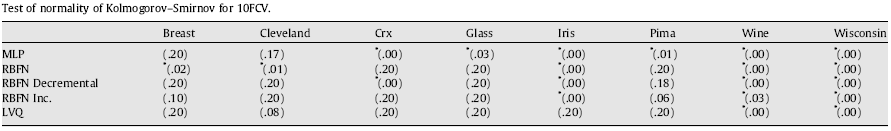

Tab. 1. Test of Normality of Kolmogorov-Smirnov for 10fcv

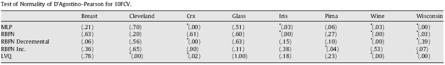
Tab. 2. Test of Normality of D’Agostino–Pearson for 10fcv

As we can observe in the run of the two tests, we can declare that the conditions needed for the application of parametric tests are not fulfilled in some cases. The normality condition is not always satisfied although the size of the sample of results would be enough (50 in this case). A main factor that influences this condition seems to be the nature of the problem, since there exist some problems in which it is never satisfied. D’Agostino–Pearson’s test is the most suitable test in these situations, where it is frequent that the sample of results would contain some ties.

In addition, we present a case study done for a given sample of results. Figure 1 presents an example of graphical representations of histograms and Q–Q graphics. An histogram represents a statistical variable by using bars, so that the area of each bar is proportional to the frequency of the represented values. A Q–Q graphic represents a confrontation between the quartiles from data observed and those from the normal distribution. In Fig. 1 we observe a common case of absolute lack of normality. The case corresponds to the run of the RBFN decremental algorithm in a Hold-Out Validation

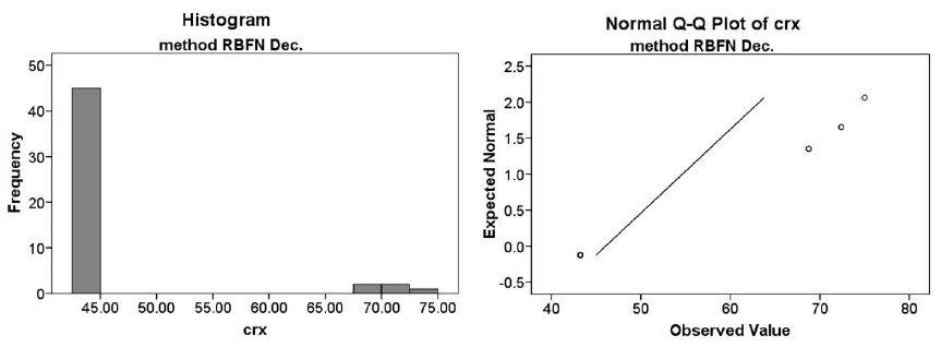
Fig. 1. Results of RBFN Decremental over crx data set in Hold-Out Validation: histogram and Q–Q graphic.

In relation to the heteroscedasticity study, next table shows the results by applying Levene’s test, where the symbol ‘*’ indicates that the variances of the distributions of the different algorithms for a certain data set are not homogeneous (we reject the null hypothesis). The homoscedasticity property is even more difficult to be fulfilled, since the variances associated to each problem also depend on the algorithm’s results, that is, the capacity of the algorithms for offering similar results with random seed variations. This fact implies that an analysis of performance of ANN methods performed through parametric statistical treatment could mean erroneous conclusions.

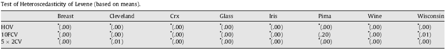
Tab. 3. Test of Homoscedasticity of Levene (based on means)

Nonparametric Tests

This section tries to describe the most used nonparametric tests in the analysis of results:

Pairwise comparisons.
Multiple comparisons with a control method.
Multiple comparisons among all methods.

Pairwise comparisons

In the discussion of the tests for comparisons of two methods over multiple cases of problems we will make two points. We shall warn against the widely used t-test as usually conceptually inappropriate and statistically unsafe. Since we will finally recommend the Wilcoxon (F. Wilcoxon. Individual comparisons by ranking methods. Biometrics, 1:80–83, 1945) signed-ranks test, it will be presented with more details. Another, even more rarely used test is the sign test which is weaker than the Wilcoxon test but also has its distinct merits. The other message will be that the described statistics measure differences between the methods from different aspects, so the selection of the test should be based not only on statistical appropriateness but also on what we intend to measure.

The Sign Test

A popular way to compare the overall performances of algorithms is to count the number of cases on which an algorithm is the overall winner. When multiple algorithms are compared, pairwise comparisons are sometimes organized in a matrix.

Some authors also use these counts in inferential statistics, with a form of binomial test that is known as the sign test Sheskin, D.J.: Handbook of Parametric and Nonparametric Statistical Procedures. CRC Press, Boca Raton (2006). If the two algorithms compared are, as assumed under the null-hypothesis, equivalent, each should win on approximately N/2 out of N problems. The number of wins is distributed according to the binomial distribution; the critical number of wins can be found in next Table. For a greater number of cases, the number of wins is under the null-hypothesis distributed according to N(N/2,SQRT(N)/2), which allows for the use of z-test: if the number of wins is at least N/2+1.96*SQRT(N)/2 (or, for a quick rule of a thumb, N/2+SQRT(N)), the
algorithm is significantly better with p < 0.05. Since tied matches support the null-hypothesis we should not discount them but split them evenly between the two methods; if there is an odd number of them, we again ignore one.

#cases	5	6	7	8	9	10	11	12	13	14	15	16	17	18	19	20	21	22	23	24	25
$\alpha = 0.05$	5	6	7	7	8	9	9	10	10	11	12	12	13	13	14	15	15	16	17	18	18
$\alpha = 0.1$	5	6	6	7	7	8	9	9	10	10	11	12	12	13	13	14	14	15	16	16	17

Table 4. Critical values for the two-tailed sign test at α = 0.05 and α = 0.1. A method is significantly better than another if it performs better on at least the cases presented in each row.

The Wilcoxon Test

Wilcoxon’s test is used for answering this question: do two samples represent two different populations? It is a non-parametric procedure employed in a hypothesis testing situation involving a design with two samples. It is the analogous of the paired t-test
in non-parametrical statistical procedures; therefore, it is a pairwise test that aims to detect significant differences between the behavior of two algorithms.

The null hypothesis for Wilcoxon’s test is H0 : θD = 0; in the underlying populations represented by the two samples of results, the median of the difference scores equals zero. The alternative hypothesis is H1 : θD ≠ 0, but also can be used H1 : θD > 0 or H1 : θD < 0 as directional hypothesis.

In the following, we describe the tests computations. Let di be the difference between the performance scores of the two algorithms on i-th out of N cases. The differences are ranked according to their absolute values; average ranks are assigned in case of ties. Let R+ be the sum of ranks for the functions on which the second algorithm outperformed the first, and R− the sum of ranks for the opposite. Ranks of di = 0 are split evenly among the sums; if there is an odd number of them, one is ignored:

$$R^+=\displaystyle\sum_{d_i>0}rank(d_i)+ \frac{1}{2} \displaystyle\sum_{d_i=0}rank(d_i)$$

$$R^-=\displaystyle\sum_{d_i>0}rank(d_i)+ \frac{1}{2} \displaystyle\sum_{d_i=0}rank(d_i)$$

Let T be the smallest of the sums, $T = min(R^+,R^−)$. If T is less than or equal to the value of the distribution of Wilcoxon for N degrees of freedom (Table B.12 in Zar, J.H.: Biostatistical Analysis. Prentice Hall, Englewood Cliffs (1999)), the null hypothesis of equality of means is rejected.

The obtaining of the p-value associated to a comparison is performed by means of the normal approximation for the Wilcoxon T statistic (Section VI, Test 18 in Sheskin, D.J.: Handbook of Parametric and Nonparametric Statistical Procedures. CRC Press, Boca Raton (2006) . Furthermore, the computation of the p-value for this test is usually included in well-known statistical software packages (SPSS, SAS, R, etc.).

Multiple comparisons with a control method

Wilcoxon’s test performs individual comparisons between two algorithms (pairwise comparisons). The p-value in a pairwise comparison is independent from another one. If we try to extract a conclusion involving more than one pairwise comparison
in a Wilcoxon’s analysis, we will obtain an accumulated error coming from the combination of pairwise comparisons. In statistical terms, we are losing the control on the Family Wise Error Rate (FWER), defined as the probability of making one or more false discoveries among all the hypotheses when performing multiple pairwise tests. The true statistical significance for combining pairwise comparisons is given by:

$$p=P(Reject H_0 \ H_0 true)$$

$$=1-P(Acept H_0|H_0 true)$$

$$=1-P(Acept A_k = A_i , i=1,...,k-1|H_0 true)$$

$$=1-\prod_{i=1}^{k-1} P(Accepts A_k = A_i |H_0 true)$$

$$=1-\prod_{i=1}^{k-1} [1-P(Reject A_k = A_i |H_0 true)]$$

$$=1-\prod_{i=1}^{k-1}(1-p_{H_i})$$

So, a pairwise comparison test, such as Wilcoxon's test, should not be used to conduct various comparisons involving a set of algorithms, because the FWER is not controlled. The expresion defined above computes the true significance obtained after performing several comparisons, hence the level of significance cannot be set before performing the comparisons and the statistical significance cannot be known a priori.

In order to carry out a comparison which involves more than two methods, under the assumption of being significance at a certain level of significance, established previously to the statistical analysis, the multiple comparisons tests should be used. In this part, we describe the most used test for performing multiple test comparisons together with a set of post-hoc procedures to compare a control method with other methods (1 x n comparisons). We refer to the Friedman Test and derivatives.

Multiple Sign Test

The multiple sign test, allows us to compare all of the other algorithms with a control labeled algorithm. It carries out the following steps:

Represent by $x_{i1} sub > and x_{ij}$ the performances of the control and the jth classifier in the ith data set.
Compute the signed differences $d_{ij} = x_{ij} - x_{i1}$. In other words, pair each performance with the control and, in each data set, subtract the control performance from the jth classifier.
Let $r_j$ equal the number of differences, $d_{ij}$, that have the less frequently occurring sign (either positive or negative) within a pairing of an algorithm with the control.
Let $M_1$ be the median response of a sample of results of the control method and $M_j$ be the median response of a sample of results of the jth algorithm. Apply one of the following decision rules:
- For testing $H_0 : M_j \ge M_1$ against $H_1 : M_j < M_1$, reject $H_0$ if the number of plus signs is less than or equal to the critical value of $R_j$ appearing in Table A.1 in (S. García, A. Fernández, J. Luengo, F. Herrera, Advanced nonparametric tests for multiple comparisons in the design of experiments in computational intelligence and data mining: Experimental Analysis of Power. Information Sciences 180 (2010) 2044–2064.) for k - 1 (number of algorithms excluding control), n and the chosen experimentwise error rate.
- For testing $H_0 : M_j \ge M_1$ against $H_1 : M_j > M_1$, reject $H_0$ if the number of minus signs is less than or equal to the critical value of Rj appearing in Table A.1 in (S. García, A. Fernández, J. Luengo, F. Herrera, Advanced nonparametric tests for multiple comparisons in the design of experiments in computational intelligence and data mining: Experimental Analysis of Power. Information Sciences 180 (2010) 2044–2064.) for k - 1; n and the chosen experimentwise error rate.

Contrast Estimation based on Medians

Using the data resulting from the run of various classifiers over multiple data sets in an experiment, the researcher could be interested in the estimation of the difference between two classifiers’ performance. A procedure for this purpose assumes that the expected differences between performances of algorithms are the same across data sets. We assume that the performance is reflected by the magnitudes of the differences between the performances of the algorithms. Consequently, we are interested in estimating the contrast between medians of samples of results considering all pairwise comparisons. It obtains a quantitative difference computed through medians between two algorithms over multiple
data sets, but the value obtained will change when using other data sets in the experiment.

It carries out the following steps:

For every pair of k algorithms in the experiment, we compute the difference between the performances of the two algorithms in each of the n data sets. In other words, we compute the differences

$$D_{i_{(uv)}}=X_{iu}-X_{iv}$$

where i = 1; ... ; n; u = 1; ... ; k; and v = 1; ... ; k. We form performance pairs only for those in which u < v.

We find the median of each set of differences and call it Zuv . We call Zuv the unadjusted estimator of $M_u - M_v . Since Z_{vu} = Z_{uv}$ , we have only to calculate $Z_{uv}$ for the case where u < v. There are k(k - 1)/2 of these medians. Also note that $Z_{uu}$ = 0.
We compute the mean of each set of unadjusted medians having the same first subscript and call the result mu; that is, we compute

$$m_u=\frac{\sum_{j=1}^{k}Z_{uj}}{k}, u=1,...,k$$

The estimator of $M_u - M_v is m_u - m_v$, where u and v range from 1 through k. For example, the difference between $M_1 and M_2 is m_1 - m_2$.

The Friedman Test

Friedman’s test is used for answering this question: In a set of k samples (where k ≥ 2), do at least two of the samples represent populations with different median values? It is a non-parametric procedure employed in a hypothesis testing situation involving a design with two or more samples. It is the analogous of the repeatedmeasures ANOVA in non-parametrical statistical procedures; therefore, it is a multiple comparison test that aims to detect significant differences between the behavior of two or more algorithms.

The null hypothesis for Friedman’s test is $H_0 : θ_1 = θ_2 = ··· = θ_k$ ; the median of the population i represents the median of the population j , i ≠ j, 1 ≤ i ≤ k, 1 ≤ j ≤ k. The alternative hypothesis is $H_1$ : Not $H_0$, so it is non-directional.

Next, we describe the tests computations. It computes the ranking of the observed results for algorithm ($r_j$ for the algorithm j with k algorithms) for each function, assigning to the best of them the ranking 1, and to the worst the ranking k. Under the null hypothesis, formed from supposing that the results of the algorithms are equivalent and, therefore, their rankings are also similar, the Friedman’s statistic

$$X_F^2=\frac{12N}{k(k+1)º}\left [ \sum_j R_j^2- \frac{k(k+1)^2}{4} \right ]$$

is distributed according to $x_F^2$ with k − 1 degrees of freedom, being $R_j = \sum_i r_i^j$, and N the number of cases of the problem considered. The critical values for the Friedman’s statistic coincide with the established in the $χ^2$ distribution when N > 10 and k > 5.

The Iman and Davenport Test

man and Davenport (Iman, R.L., Davenport, J.M.: Approximations of the critical region of the Friedman statistic. Commun. Stat. 18, 571–595 (1980)) proposed a derivation from the Friedman’s statistic given that this last metric produces a conservative undesirably effect. The proposed statistic is

$F_F=\frac{(N-1)X_F^2}{N(k-1)-X_F^2}

and it is distributed according to a F distribution with k − 1 and (k − 1)(N − 1) degrees of freedom.

Computation of the p-values given a $χ^2 or F_F$ statistic can be done by using the algorithms in Abramowitz, M.: Handbook of Mathematical Functions, With Formulas, Graphs, and Mathematical Tables. Dover, New York (1974). Also, most of the statistical software packages include it.

The rejection of the null hypothesis in both tests described above does not involve the detection of the existing differences among the algorithms compared. They only inform us about the presence of differences among all samples of results compared. In order to conducting pairwise comparisons within the framework of multiple comparisons, we can proceed with a post-hoc procedure. In this case, a control algorithm (maybe a proposal to be compared) is usually chosen. Then, the post-hoc procedures proceed to compare the control algorithm with the remain k − 1 algorithms. Next, we describe three post-hoc procedures:

Friedman Aligned Ranks Test

The Friedman test is based on n sets of ranks, one set for each data set in our case; and the performances of the algorithms analyzed are ranked separately for each data set. Such a ranking scheme allows for intra-set comparisons only, since inter-set comparisons are not meaningful. When the number of algorithms for comparison is small, this may pose a disadvantage. In such cases, comparability among data sets is desirable and we can employ the method of aligned ranks (J.L. Hodges, E.L. Lehmann, Ranks methods for combination of independent experiments in analysis of variance, Annals of Mathematical Statistics 33 (1962) 482–497).

In this technique, a value of location is computed as the average performance achieved by all algorithms in each data set. Then, it calculates the difference between the performance obtained by an algorithm and the value of location. This step is repeated for algorithms and data sets. The resulting differences, called aligned observations, which keep their identities with respect to the data set and the combination of algorithms to which they belong, are then ranked from 1 to kn relative to each other. Then, the ranking scheme is the same as that employed by a multiple comparison procedure which employs independent samples; such as the Kruskal–Wallis test. The ranks assigned to the aligned observations are called aligned ranks.

The Friedman Aligned Ranks test statistic can be written as

$$T=\frac{(k-1)[\sum_{j=1}^k \widehat{R_{.j}^2}-(kn^2/4)(kn+1)^2]}{{[kn(kn+1)(2kn+1)]/6}-(1/k)\sum_{i=1}^n \widehat{R_{i.}^2}}$$

where $R_i$. is equal to the rank total of the ith data set and $R_{.j}$ is the rank total of the jth algorithm.

The test statistic T is compared for significance with a chi-square distribution for k - 1 degrees of freedom. Critical values can be found at Table A3 in (Sheskin, D.J.: Handbook of Parametric and Nonparametric Statistical Procedures. CRC Press, Boca Raton (2006)). Furthermore, the p-value could be computed through normal approximations (Abramowitz, M.: Handbook of Mathematical Functions, With Formulas, Graphs, and Mathematical Tables. Dover, New York (1974)). If the null hypothesis is rejected, we can proceed with a post hoc test.

Quade Test

The Friedman test considers all data sets to be equal in terms of importance. An alternative to this could take into account the fact that some data sets are more difficult or the differences registered on the run of various algorithms over them are larger. The rankings computed on each data set could be scaled depending on the differences observed in the algorithms’ performances. The Quade test conducts a weighted ranking analysis of the sample of results (D. Quade, Using weighted rankings in the analysis of complete blocks with additive block effects, Journal of the American Statistical Association 74 (1979) 680–683.).

The procedure starts finding the ranks $r_i^j$ in the same way as the Friedman test does. The next step requires the original values of performance of the classifiers $x_{ij}$. Ranks are assigned to the data sets themselves according to the size of the sample range in each data set. The sample range within data set i is the difference between the largest and the smallest observations within that data set:

$$Range in data set: i=\displaystyle max_j{x_{ij}-\displaystyle min_j{x_{ij}}}$$

Obviously, there are n sample ranges, one for each data set. Assign rank 1 to the data set with the smallest range, rank 2 to the second smallest, and so on to the data set with the largest range, which gets rank n. Use average ranks in case of ties. Let $Q_1,Q_2, ... ,Q_n$ be the ranks assigned to data sets 1, 2, ... , n, respectively.

Finally, the data set rank $Q_i$ is multiplied by the difference between the rank within data set i, $r^j_i$ , and the average rank within data sets, (k + 1) / 2, to get the product $S_{ij}, where

$$S_{ij}=Q_i \left [ r^j_i- \frac{k+1}{2} \right ]$$

is a statistic that represents the relative size of each observation within the data set, adjusted to reflect the relative significance of the data set in which it appears.

For convenience and to establish a relationship with the Friedman test, we will also use rankings without average adjusting:

$$W_{ij}=Q\left [ r^j_i \right ]$$

Let $S_j$ denote the sum for each classifier,

$$S_j=\sum_{i=1}^n S_{ij} and W_j = \sum_{i=1}^n W_{ij}, for j = 1,2,...,k.$$

Next we must to calculate the terms:

$$$A_2=n(n+1)(2n+1)(k)(k+1)(k-1)/72$$

$$B=\frac{1}{n} \displaystyle\sum_{j=1}^k S_j^2$$

The test statistic is

$$T_3=\frac{(n-1)B}{A_2-B}

which is distributed according to the F-distribution with k - 1 and (k - 1)(n - 1) degrees of freedom. The table of critical values for the F-distribution is given in Table A10 in Sheskin, D.J.: Handbook of Parametric and Nonparametric Statistical Procedures. CRC Press, Boca Raton (2006). Moreover, the p-value could be computed through normal approximations (Abramowitz, M.: Handbook of Mathematical Functions, With Formulas, Graphs, and Mathematical Tables. Dover, New York (1974)). If $A_2 = B$, consider the point to be in the critical region of the statistical distribution and calculate the p-value as $(1/k!)^{n-1}$. If the null hypothesis is rejected, we can proceed with a post hoc test.

Post-hoc Procedures

We focus on the comparison between a control method, which is usually the proposed method, and a set of algorithms used in the empirical study. This set of comparisons is associated with a set or family of hypotheses, all of which
are related to the control method. Any of the post hoc tests is suitable for application to nonparametric tests working over a family of hypotheses. The test statistic for comparing the ith algorithm and jth algorithm depends on the main nonparametric procedure used:

Friedman test: In (Zar, J.H.: Biostatistical Analysis. Prentice Hall, Englewood Cliffs (1999)) we can see that the expression for computing the test statistic in Friedman test is:

$$Z=(R_i-R_j)/\sqrt{\frac{k(k+1)}{6n}}$$

where $R_i; R_j$ are the average rankings by Friedman of the algorithms compared.

Friedman Aligned Ranks test: Since the set of related rankings is converted to absolute rankings, the expression for computing the test statistic in Friedman Aligned Ranks is the same as that used by the Kruskal–Wallis test (Zar, J.H.: Biostatistical Analysis. Prentice Hall, Englewood Cliffs (1999)):

$$Z=(\widehat{R_i}-\widehat{R_j})/\sqrt{\frac{k(nk+1)}{6}}$$

where $R_i; R_j$ are the average rankings by Friedman Aligned Ranks of the algorithms compared.

Quade test: In (W.J. Conover, Practical Nonparametric Statistics, John Wiley and Sons, (1999)) the test statistic for comparing two algorithms is given by using the t-student distribution, but we can easily obtain the equivalent in a normal distribution N(0,1):

$$Z=(T_i-T_j)/\sqrt{\frac{k(k+1)(2n+1)(k-1)}{18n(n+1)}}$$

where $T_i=\frac{W_i}{n(n+1)/2}$, $T_j=\frac{W_j}{n(n+1)/2}$, and $W_i$ and $W_j$ are the rankings without average adjusting by Quade of the algorithms compared. In fact, $T_i$ and $T_j$ compute the correct average magnitudes.

In statistical hypothesis testing, the p-value is the probability of obtaining a result at least as extreme as the one that was actually observed, assuming that the null hypothesis is true. It is a useful and interesting datum for many consumers of statistical analysis. A p-value provides information about whether a statistical hypothesis test is significant or not, and it also indicates something about ‘‘how significant” the result is: the smaller the p-value, the stronger the evidence against the null hypothesis. Most importantly, it does this without committing to a particular level of significance.

When a p-value is considered in a multiple comparison, it reflects the probability error of a certain comparison, but it does not take into account the remaining comparisons belonging to the family. If one is comparing k algorithms and in each comparison the level of significance is α, then in a single comparison the probability of not making a Type I error is (1-α), then the probability of not making a Type I error in the k - 1 comparison is $(1 - α)^{(k - 1)}$. Then the probability of making one or more Type I error is $1 - (1 - α)^{(k - 1)}$.

One way to solve this problem is to report adjusted p-values (APVs) which take into account that multiple tests are conducted. An APV can be compared directly with any chosen significance level α. We recommend the use of APVs due to the fact that they provide more information in a statistical analysis.

Adjusted p-values

The z value in all cases is used to find the corresponding probability (p-value) from the table of normal distribution N(0,1), which is then compared with an appropriate level of significance a (Table A1 in Sheskin, D.J.: Handbook of Parametric and Nonparametric Statistical Procedures. CRC Press, Boca Raton (2006)). The post hoc tests differ in the way they adjust the value of a to compensate for multiple comparisons.

Next, we will define a candidate set of post hoc procedures and we will explain how to compute the APVs depending on the post hoc procedure used in the analysis, following the indications given in P.H. Westfall, S.S. Young, Resampling-based Multiple Testing: Examples and Methods for p-Value Adjustment, John Wiley and Sons (2004). The notation used in the computation of the APVs is as follows:

Indexes i and j each correspond to a concrete comparison or hypothesis in the family of hypotheses, according to an incremental order of their p-values. Index i always refers to the hypothesis in question whose APV is being computed and index j refers to another hypothesis in the family.
$p_j$ is the p-value obtained for the jth hypothesis.
k is the number of classifiers being compared.

The procedures of p-value adjustment can be classified into:

one-step
- The Bonferroni–Dunn procedure (Dunn–Sidak approximation) (O.J. Dunn, Multiple comparisons among means, Journal of the American Statistical Association 56 (1961) 52–64): it adjusts the value of a in a single step by dividing the value of a by the number of comparisons performed, (k - 1). This procedure is the simplest but it also has little power.Bonferroni $APV_i: min{v; 1}, where v = (k - 1)p_i$.
step-down
- The Holm procedure (S. Holm, A simple sequentially rejective multiple test procedure, Scandinavian Journal of Statistics 6 (1979) 65–70): it adjusts the value of a in a step-down manner. Let $p_1; p_2; ... ; p_{k-1}$ be the ordered p-values (smallest to largest), so that $p_1 ≤ p_2 ≤ ... ≤ p_{k-1}$, and $H_1;H_2; ... ;H_{k-1}$ be the corresponding hypotheses. The Holm procedure rejects $H_1 to H_{i-1}$ if i is the smallest integer such that $p_i > α/(k - 1)$. Holm’s step-down procedure starts with the most significant p-value. If $p_1$ is below α/(k - 1), the corresponding hypothesis is rejected and we are allowed to compare $p_2$ with α/(k - 2). If the second hypothesis is rejected, the test proceeds with the third, and so on. As soon as a certain null hypothesis cannot be rejected, all the remaining hypotheses are retained as well. Holm $APV_i$: min{v; 1}, where v = max{(k - j)$p_j$ : 1 ≤ j ≤ i}
- The Holland procedure (B.S. Holland, M.D. Copenhaver, An improved sequentially rejective Bonferroni test procedure, Biometrics 43 (1987) 417–423): it also adjusts the value of a in a step-down manner, as Holm’s method does. It rejects $H_1$ to $H_{i - 1}$ if i is the smallest integer so that $p_i > 1 - (1 - α)^{1/({k - i})}$.Holland $APV_i$: min{v; 1}, where $v = max(1 - (1 - p_j)^{k - j} : 1 ≤ j ≤ i)$.
- The Finner procedure (H. Finner, On a monotonicity problem in step-down multiple test procedures, Journal of the American Statistical Association 88 (1993) 920–923): it also adjusts the value of a in a step-down manner, as Holm’s or Holland’s method do. It rejects $H_1$ to $H_{i - 1}$ if i is the smallest integer so that $pi > 1 - (1 - α)^{i/(k - 1)}$ . Finner $APV_i$: min{v; 1}, where $v = max(1 - (1 - p_j)^{(k - 1)}/j : 1 ≤ j ≤ i($.
step-up
- The Hochberg procedure (Y. Hochberg, A sharper Bonferroni procedure for multiple tests of significance, Biometrika 75 (1988) 800–803) it adjusts the value of a in a step-up manner. Hochberg’s step-up procedure works in the opposite direction, comparing the largest p value with a, the next largest with α=2, the next with α=3, and so forth until it encounters a hypothesis it can reject. All hypotheses with smaller p-values are then rejected as well. Hochberg $APV_i: max{(k - j)p_j : (k - 1) ≥ j ≥ i}$
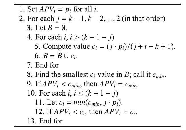
- The Hommel procedure (G. Hommel, A stagewise rejective multiple test procedure based on a modified Bonferroni test, Biometrika 75 (1988) 383–386) is more complicated to compute and understand. First, we need to find the largest j for which $p_{n - j + k}$ > kα/j for all k = 1, ..., j. If no such j exists, we can reject all hypotheses, otherwise we reject all for which $p_i ≤ α/j$. Hommel $APV_i$: see next algorithm:
- The Rom procedure (D.M. Rom, A sequentially rejective test procedure based on a modified Bonferroni inequality, Biometrika 77 (1990) 663–665): Rom developed a modification to Hochberg’s procedure to increase its power. It works in exactly the same way as the Hochberg procedure, except that the a values are computed through the expression:
- $$\alpha_{k-i}=[\sum_{j=1}^{i-1} \alpha^j - \sum_{j=1}^{i-2} \binom{i}{j} \alpha_{k-1-j}^{i-j}]/i$$
- where $α_{k - 1} = α$ and $α_{k - 2} = α/2$. Rom $APV_i : max{(r_{k - j})p_j : (k - 1) ≥ j ≥ i}$, where $r_{k - j}$ can be obtained from previous Eq. (r = {1, 2, 3, 3.814, 4.755, 5.705, 6.655, ...}).
two-step
- The Li procedure (J. Li, A two-step rejection procedure for testing multiple hypotheses, Journal of Statistical Planning and Inference 138 (2008) 1521–1527): Li proposed a two-step rejection procedure. Step 1: Reject all $H_i$ if $p_{k - 1} ≤ α$. Otherwise, accept the hypothesis associated to $p_{k - 1} and go to Step 2. Step 2: Reject any remaining $H_i$ with $p_i ≤(1 - p_{k - 1})/(1 - α)α$. Li $APV_i : p_i/(p_i + 1 -p_{k - 1})$.

Multiple comparisons among all methods

Friedman’s test is an omnibus test which can be used to carry out these types of comparison. It allows to detect differences considering the global set of classifiers. Once Friedman’s test rejects the null hypothesis, we can proceed with a post-hoc test in order to find the concrete pairwise comparisons which produce differences. Before, we focused on procedures that control the family-wise error when comparing with a control classifier, arguing that the objective of a study is to test whether a newly proposed method is better than the existing ones. For this reason, we have described and studied procedures such as Bonferroni-Dunn, Holm’s and Hochberg’s methods.

When our interest lies in carrying out a multiple comparison in which all possible pairwise comparisons need to be computed (n x n comparison), the classic procedure that can be used is the Nemenyi procedure (P. B. Nemenyi. Distribution-free Multiple comparisons. PhD thesis, Princeton University, 1963). It adjusts the value of a in a single step by dividing the value of α by the number of comparisons performed, m = k(k−1)=2. This procedure is the simplest but it also has little power.

The hypotheses being tested belonging to a family of all pairwise comparisons are logically interrelated so that not all combinations of true and false hypotheses are possible. As a simple example of such a situation suppose that we want to test the three hypotheses of pairwise equality associated with the pairwise comparisons of three classifiers $C_i$; i = 1, 2, 3. It is easily seen from the relations among the hypotheses that if any one of them is false, at least one other must be false. For example, if $C_1$ is better/worse than $C_2$, then it is not possible that $C_1$ has the same performance as $C_3$ and $C_2$ has the same performance as $C_3. C_3$ must be better/worse than $C_1$ or $C_2$ or the two classifiers at the same time. Thus, there cannot be one false and two true hypotheses among these three.

Based on this argument, Shaffer proposed two procedures which make use of the logical relation among the family of hypotheses for adjusting the value of α (J.P. Shaffer. Modified sequentially rejective multiple test procedures. Journal of the American Statistical Association, 81(395):826–831, 1986.).

Shaffer’s static procedure: following Holm’s step down method, at stage j, instead of rejecting $H_i$ if $p_i$ ≤ α /(m − i + 1), reject $H_i$ if $p_i$ ≤ α / $t_i$, where $t_i$ is the maximum number of hypotheses which can be true given that any (i − 1) hypotheses are false. It is a static procedure, that is, $t_1$, ..., $t_m$ are fully determined for the given hypotheses $H_1$, ..., $H_m$, independent of the observed p-values. The possible numbers of true hypotheses, and thus the values of $t_i$ can be obtained from the recursive formula

$$S(k)=\displaystyle\bigcup_{j=1}^{k}{\binom{j}{2}+x:x \in S(k-j)}$$

where S(k) is the set of possible numbers of true hypotheses with k methods being compared, k ≥ 2, and S(0) = S(1) = {0}.

G. Bergmann and G. Hommel. Improvements of general multiple test procedures for redundant systems of hypotheses. In P. Bauer, G. Hommel, and E. Sonnemann, editors, Multiple Hypotheses Testing, pages 100–115. Springer, Berlin, 1988 was proposed a procedure based on the idea of finding all elementary hypotheses which cannot be rejected. In order to formulate Bergmann-Hommel’s procedure, we need the following definition.

Definition 1: An index set of hypotheses I ⊆ {1, ..., m} is called exhaustive if exactly all $H_j$, j ∈ I, could be true.

Under this definition, Bergmann-Hommel procedure works as follows.

Bergmann and Hommel procedure (G. Bergmann and G. Hommel. Improvements of general multiple test procedures for redundant systems of hypotheses. In P. Bauer, G. Hommel, and E. Sonnemann, editors, Multiple Hypotheses Testing, pages 100–115. Springer, Berlin, 1988): Reject all Hj with j not in A, where the acceptance set

$$A=\bigcup{I:I exhaustive, min(P_i:i \in I) > \alpha / |I|)}$$

is the index set of null hypotheses which are retained.

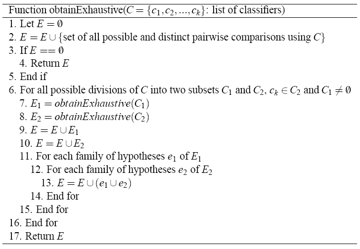
For this procedure, one has to check for each subset I of {1, ..., m} if I is exhaustive, which leads to intensive computation. Due to this fact, we will obtain a set, named E, which will contain all the possible exhaustive sets of hypotheses for a certain comparison. A rapid algorithm which was described in G. Hommel and G. Bernhard. A rapid algorithm and a computer program for multiple test procedures using procedures using logical structures of hypotheses. Computer Methods and Programs in Biomedicine, 43:213–216, 1994 allows a substantial reduction in computing time. Once the E set is obtained, the hypotheses that do not belong to the A set are rejected.

Next figure shows a valid algorithm for obtaining all the exhaustive sets of hypotheses, using as input a list of algorithms C. E is a set of families of hypotheses; likewise, a family of hypotheses is a set of hypotheses. The most important step in the algorithm is the number 6. It performs a division of the classifiers into two subsets, in which the last classifier k always is inserted in the second subset and the first subset cannot be empty. In this way, we ensure that a subset yielded in a division is never empty and no repetitions are produced.

Finally, we will explain how to compute the APVs for the three post-hoc procedures described above, following the indications given in Wright, S.P.: Adjusted p-values for simultaneous inference. Biometrics 48, 1005–1013 (1992).

Shaffer static APVi: min {v;1}, where v = max {tjpj : 1 ≤ j ≤ i}.
Bergmann-Hommel APVi: min {v;1}, where v = max {|I|·min{pj; j ∈ I} : I exhaustive; i ∈ I}.

Case Studies

In this section, two case studies will be presented in order to illustrate the use of multiple comparisons nonparametric test in Computational Intelligence and Data Mining experimentations:

Multiple comparisons with a control method.
Multiple comparisons among all methods.

Multiple comparisons with a control method.

We present a case study where four rule induction algorithms will be compared with a control method. The complete study can be found in S. García, A. Fernández, J. Luengo, F. Herrera, A Study of Statistical Techniques and Performance Measures for Genetics-Based Machine Learning: Accuracy and Interpretability. Soft Computing 13:10 (2009) 959-977, doi:10.1007/s00500-008-0392-y.

Four of them are Genetics-based Machine Learning (GBML) methods:

XCS (Wilson SW (1995) Classifier fitness based on accuracy. Evol Comput 3(2):149–175)
GASSIST-ADI (Bacardit J, Garrell JM (2007) Bloat control and generalization pressure using the minimum description length principle for Pittsburgh approach learning classifier system. In: Kovacs T, Llorá X, Takadama K (eds) Advances at the frontier of learning classifier systems, vol 4399. LNCS, USA, pp 61–80)
Pitts-GIRLA (Corcoran AL, Sen S (1994) Using real-valued genetic algorithms to evolve rule sets for classification. In: Proceedings of the IEEE conference on evolutionary computation, pp 120–124)
HIDER (Aguilar-Ruiz JS, Giráldez R, Riquelme JC (2007) Natural encoding for evolutionary supervised learning. IEEE Trans Evol Comput 11(4):466–479)

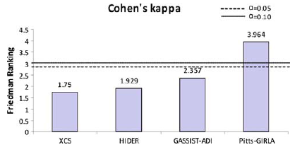
and one of them is the classic CN2 algorithm (Clark P, Niblett T (1989) The CN2 induction algorithm. Machine Learn 3(4):261–283). One of the GBML algorithms is chosen as the control algorithm, XCS (Wilson SW ( 1995) Classifier fitness based on accuracy. Evol Comput 3(2):149–175). Two performance measures are used for compariong the behaviour of the algorithms: Accuracy and Cohen's kappa (Cohen JA (1960) Coefficient of agreement for nominal scales. Educ Psychol Meas 37–46).

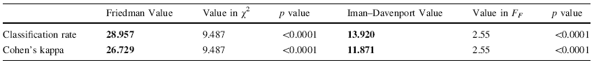
First of all, we have to test whether significant differences exist among all the mean values. The next table shows the result of applying a Friedman and Iman–Davenport tests. The table shows the Friedman and Iman–Davenport values, χF2 and FF,respectively, and it relates them with the corresponding critical values for each distribution by using a level of significance α = 0.05. The p value obtained is also reported for each test. Given that the statistics of Friedman and Iman–Davenport are clearly greater than their associated critical values, there are significant differences among the observed results with a level of significance α ≤ 0.05. According to these results, a posthoc statistical analysis is needed in the two cases.

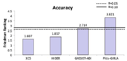
Then, we will employ a Bonferroni-Dunn test to detect significant differences for the control algorithm in each measure. It obtains the values CD = 1.493 and CD = 1.34 for α = 0.05 and α = 0.10 respectively in the two measures considered. The following figures summarize the ranking obtained by the Friedman test and draw the threshold of the critical difference of Bonferroni–Dunn’ procedure, with the two levels of significance mentioned above. They display a graphical representation composed by bars whose height is proportional to the average ranking obtained for each algorithm in each measure studied. If we choose the smallest of them (which corresponds to the best algorithm), and we sum its height with the critical difference obtained by the Bonferroni method (CD value), we represent a cut line that goes through all the graphic. Those bars which are higher than this cut line belong to the algorithms whose performance is significantly worse than that of the control algorithm.

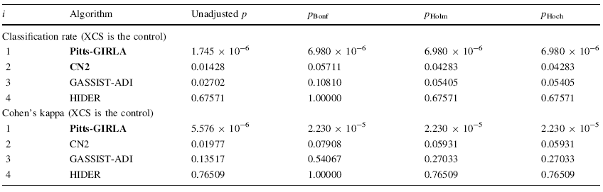
We will apply more powerful procedures, such as Holm and Hochbergs ones, for comparing the control algorithm with the rest of algorithms. The next table shows all the adjusted p values for each comparison which involves the control algorithm. The p value is indicated in each comparison and we stress in bold the algorithms which are worse than the control, considering a level of significance α = 0.05.

Taken from S. García, A. Fernández, J. Luengo, F. Herrera, Advanced nonparametric tests for multiple comparisons in the design of experiments in computational intelligence and data mining: Experimental analysis of power. Information Sciences 180 (2010) 2044–2064 doi:10.1016/j.ins.2009.12.010, we present a case study where three different computational intelligence algorithms will be compared with a control method.

The three algorithms and the control methods are:

FH-GBML (H. Ishibuchi, T. Yamamoto, T. Nakashima, Hybridization of fuzzy GBML approaches for pattern classification problems, IEEE Transactions on System, Man and Cybernetics B 35 (2) (2005) 359–365.)

IS-CHC + 1NN (J.R. Cano, F. Herrera, M. Lozano, Using evolutionary algorithms as instance selection for data reduction in KDD an experimental study, IEEE Transactions on Evolutionary Computation 7 (6) (2003) 561–575.)

NNEP (F. Martínez-Estudillo, C. Hervás-Martínez, P. Gutiérrez, A. Martínez-Estudillo, Evolutionary product-unit neural networks classifiers, Neurocomputing 72 (1–3) (2008) 548–561.)

PDFC as control method (Y. Chen, J. Wang, Support vector learning for fuzzy rule-based classification systems, IEEE Transactions on Fuzzy Systems 11 (6) (2003) 716–728)

The following tables show the results in the final form of APVs for the experimental study considered in this case. As we can see, this example is suitable for observing the difference of power among the test procedures. Also, these tables can provide information about the state of retention or rejection of any hypothesis, comparing its associated APV with the level of significance fixed at the beginning of the statistical analysis.

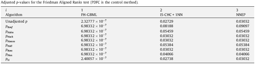
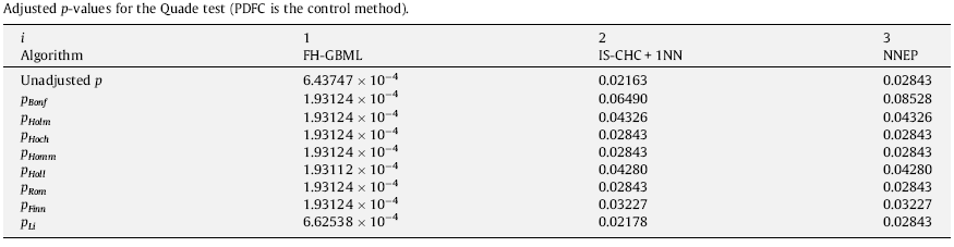
First of all, we can observe that the Bonferroni procedure obtains the highest APV. Theoretically, the step-down procedures usually have less power than step-up ones and the Li procedure seems to be the multiple comparison test with highest power. On the other hand, referring to a comparison between multiple comparison nonparametric tests; that is, Friedman, Friedman Aligned Ranks and Quade; we can see that Quade’s procedure is the one which obtains the lowest unadjusted p-value in this example.

Multiple comparisons among all methods.

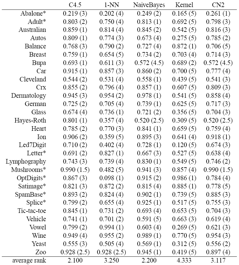
Taken from the paper S. García, F. Herrera, An Extension on "Statistical Comparisons of Classifiers over Multiple Data Sets" for all Pairwise Comparisons. Journal of Machine Learning Research 9 (2008) 2677-2694, this case study show an example involving the four procedures of all pairwise comparison described with a comparison of five classifiers:

C4.5 (J. R. Quinlan. Programs for Machine Learning. Morgan Kauffman, 1993)
One Nearest Neighbor (1-NN) with Euclidean distance
NaiveBayes
Kernel (G. J. McLachlan. Discriminant Analysis and Statistical Pattern Recognition. Wiley Series in Probability and Mathematical Statistics, 2004)
CN2 (P. Clark and T. Niblett. The CN2 induction algorithm. Machine Learning, 3(4):261–283, 1989)

We have used 10-fold cross validation and standard parameters for each algorithm. The results correspond to average accuracy or 1 − class_error in test data. We have used 30 data sets. Next table shows the overall process of computation of average rankings.

Friedman and Iman and Davenport tests check whether the measured average ranks are significantly different from the mean rank R_j = 3. They respectively use the χ² and the F statistical distributions to determine if a distribution of observed frequencies differs from the theoretical expected frequencies. Their statistics use nominal (categorical) or ordinal level data, instead of using means and variances. Demsar (2006) detailed the computation of the critical values in each distribution. In this case, the critical values are 9.488 and 2.45, respectively at α = 0.05, and the Friedman’s and Iman-Davenport’s statistics are:

$$X_F^2 = 39.647; F_F = 14.309.$$

Due to the fact that the critical values are lower than the respective statistics, we can proceed with the post-hoc tests in order to detect significant pairwise differences among all the classifiers. For this, we have to compute and order the corresponding statistics and p-values. The standard error in the pairwise comparison between two classifiers is SE = 0.408. The following table presents the family of hypotheses ordered by their p-value and the adjustment of a by Nemenyi’s, Holm’s and Shaffer’s static procedures.

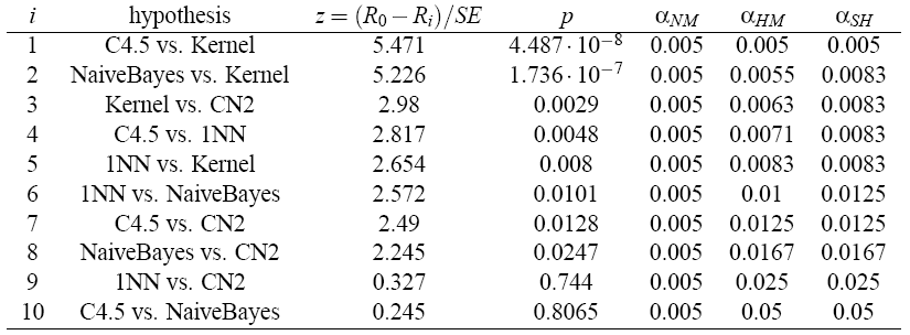
Nemenyi’s test rejects the hypotheses [1–4] since the corresponding p-values are smaller than the adjusted α’s.
Holm’s procedure rejects the hypotheses [1–5].
Shaffer’s static procedure rejects the hypotheses [1–6].
Bergmann-Hommel’s dynamic procedure first obtains the exhaustive index set of hypotheses. It obtains 51 index sets. From the index sets, it computes the A set. It rejects all hypotheses Hj with j not in A, so it rejects the hypotheses [1–8].

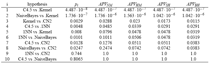
Next table shows the results in the final form of APVs for the example considered in this section. As we can see, this example is suitable for observing the difference of power among the test procedures. Also, this table can provide information about the state of retainment or rejection of any hypothesis, comparing its associated APV with the level of significance previously fixed.

Considerations and Recommendations on the Use of Nonparametric Tests

This section remarks some considerations and recommendations about Nonparametric tests when they are used over any type of comparison.

Considerations on the use of Nonparametric Tests.

Pairwise comparisons.
Multiple comparisons with a control method.

Pairwise comparisons.

Although Wilcoxon’s test and the remaining post-hoc tests for multiple comparisons belong to the non-parametric statistical tests, they operate in a different way. The main difference lies in the computation of the ranking. Wilcoxon’s test computes a ranking based on differences between case problems independently, whereas Friedman and derivative procedures compute the ranking between algorithms. (S. García, A. Fernández, J. Luengo, F. Herrera, A Study of Statistical Techniques and Performance Measures for Genetics-Based Machine Learning: Accuracy and Interpretability. Soft Computing 13:10 (2009) 959-977) (S. García, D. Molina, M. Lozano, F. Herrera, A Study on the Use of Non-Parametric Tests for Analyzing the Evolutionary Algorithms' Behaviour: A Case Study on the CEC'2005 Special Session on Real Parameter Optimization. Journal of Heuristics, 15 (2009) 617-644)

In relation to the sample size (number of case problems when performing Wilcoxon’s or Friedman’s tests in multiple-problem analysis), there are two main aspects to be determined. Firstly, the minimum sample considered acceptable for each test needs to be stipulated. There is no established agreement about this specification. Statisticians have studied the minimum sample size when a certain power of the statistical test is expected. In our case, the employment of a, as large as possible, sample size is preferable, because the power of the statistical tests (defined as the probability that the test will reject a false null hypothesis) will increase. Moreover, in a multiple-problem analysis, the increasing of the sample size depends on the availability of new case problems (which should be well-known in computational intelligence or data mining field). Secondly, we have to study how the results are expected to vary if there was a larger sample size available. In all statistical tests used for comparing two or more samples, the increasing of the sample size benefits the power of the test. In the following items, we will state that Wilcoxon’s test is less influenced by this factor than Friedman’s test. Finally, as a rule of thumb, the number of case problems (N) in a study should be N = a · k, where k is the number of algorithms to be compared and a ≥ 2. (S. García, A. Fernández, J. Luengo, F. Herrera, A Study of Statistical Techniques and Performance Measures for Genetics-Based Machine Learning: Accuracy and Interpretability. Soft Computing 13:10 (2009) 959-977) (S. García, D. Molina, M. Lozano, F. Herrera, A Study on the Use of Non-Parametric Tests for Analyzing the Evolutionary Algorithms' Behaviour: A Case Study on the CEC'2005 Special Session on Real Parameter Optimization. Journal of Heuristics, 15 (2009) 617-644)

Taking into account the previous observation and knowing the operations performed by the non-parametric tests, we can deduce that Wilcoxon’s test is influenced by the number of case problems used. On the other hand, both the number of algorithms and case problems are crucial when we refer to the multiple comparisons tests (such as Friedman’s test), given that all the critical values depend on the value of N (see expressions above). However, the increasing/decreasing of the number of case problems rarely affects in the computation of the ranking. In these procedures, the number of functions used is an important factor to be considered when we want to control the FWER. (S. García, A. Fernández, J. Luengo, F. Herrera, A Study of Statistical Techniques and Performance Measures for Genetics-Based Machine Learning: Accuracy and Interpretability. Soft Computing 13:10 (2009) 959-977) (S. García, D. Molina, M. Lozano, F. Herrera, A Study on the Use of Non-Parametric Tests for Analyzing the Evolutionary Algorithms' Behaviour: A Case Study on the CEC'2005 Special Session on Real Parameter Optimization. Journal of Heuristics, 15 (2009) 617-644)

Multiple Comparisons with a control method.

A multiple comparison of various algorithms must be carried out first by using a statistical method for testing the differences among the related samples means, that is, the results obtained by each algorithm. Once this test rejects the hypothesis of equivalence of means, the detection of the concrete differences among the algorithms can be done with the application of post-hoc statistical procedures, which are methods used for comparing a control algorithm with two or more algorithms. (S. García, A. Fernández, J. Luengo, F. Herrera, A Study of Statistical Techniques and Performance Measures for Genetics-Based Machine Learning: Accuracy and Interpretability. Soft Computing 13:10 (2009) 959-977) (S. García, D. Molina, M. Lozano, F. Herrera, A Study on the Use of Non-Parametric Tests for Analyzing the Evolutionary Algorithms' Behaviour: A Case Study on the CEC'2005 Special Session on Real Parameter Optimization. Journal of Heuristics, 15 (2009) 617-644)

An appropriate number of algorithms in contrast with an appropriate number of case problems are needed to be used in order to employ each type of test. The number of algorithms used in multiple comparisons procedures must be lower than the number of case problems. In general, p-values are lower agreeing with the increasing of the number of case problems used in multiple comparison procedures; therefore, the differences among the algorithms are more detectable. (S. García, A. Fernández, J. Luengo, F. Herrera, A Study of Statistical Techniques and Performance Measures for Genetics-Based Machine Learning: Accuracy and Interpretability. Soft Computing 13:10 (2009) 959-977) (S. García, D. Molina, M. Lozano, F. Herrera, A Study on the Use of Non-Parametric Tests for Analyzing the Evolutionary Algorithms' Behaviour: A Case Study on the CEC'2005 Special Session on Real Parameter Optimization. Journal of Heuristics, 15 (2009) 617-644)

As we have suggested, multiple comparison tests must be used when we want to establish a statistical comparison of the results reported among various algorithms. We focus in cases when a method is compared against a set of algorithms. It could be carried out first by using a statistical method for testing the differences among the related samples means, that is, the results obtained by each algorithm. There are three alternatives: the Friedman test with the Iman–Davenport extension, the Friedman Aligned Ranks test and the Quade test. Once one of these tests rejects the hypothesis of equivalence of medians, the detection of the specific differences among the algorithms can be made with the application of post hoc statistical procedures, which are methods used for specifically comparing a control algorithm with two or more algorithms. (S. García, A. Fernández, J. Luengo, F. Herrera, Advanced nonparametric tests for multiple comparisons in the design of experiments in computational intelligence and data mining: Experimental Analysis of Power. Information Sciences 180 (2010) 2044–2064. doi:10.1016/j.ins.2009.12.010.)

Recommendations on the use of Nonparametric Tests

Pairwise comparisons.
Multiple comparisons with a control method.
Multiple comparisons among all methods.

Pairwise comparisons.

An appropriate number of algorithms in contrast with an appropriate number of case problems are needed to be used in order to employ each type of test. The number of algorithms used in multiple comparisons procedures must be lower than the number of case problems. The previous statement may not be true in Wilcoxon’s test. The influence of the number of case problems used is more noticeable in multiple comparisons procedures than in Wilcoxon’s test. (S. García, A. Fernández, J. Luengo, F. Herrera, A Study of Statistical Techniques and Performance Measures for Genetics-Based Machine Learning: Accuracy and Interpretability. Soft Computing 13:10 (2009) 959-977) (S. García, D. Molina, M. Lozano, F. Herrera, A Study on the Use of Non-Parametric Tests for Analyzing the Evolutionary Algorithms' Behaviour: A Case Study on the CEC'2005 Special Session on Real Parameter Optimization. Journal of Heuristics, 15 (2009) 617-644)

Multiple comparisons with a control method.

Holm’s procedure can always be considered better than Bonferroni-Dunn’s one, because it appropriately controls the FWER and it is more powerful than the Bonferroni-Dunn’s. We strongly recommend the use of Holm’s method in a rigorous comparison. Nevertheless, the results offered by the Bonferroni-Dunn’s test are suitable to be visualized in graphical representations. (S. García, A. Fernández, J. Luengo, F. Herrera, A Study of Statistical Techniques and Performance Measures for Genetics-Based Machine Learning: Accuracy and Interpretability. Soft Computing 13:10 (2009) 959-977) (S. García, D. Molina, M. Lozano, F. Herrera, A Study on the Use of Non-Parametric Tests for Analyzing the Evolutionary Algorithms' Behaviour: A Case Study on the CEC'2005 Special Session on Real Parameter Optimization. Journal of Heuristics, 15 (2009) 617-644)

Hochberg’s procedure is more powerful than Holm’s. The differences reported between it and Holm’s procedure are in practice rather small. We recommend the use of this test together with Holm’s method. (S. García, A. Fernández, J. Luengo, F. Herrera, A Study of Statistical Techniques and Performance Measures for Genetics-Based Machine Learning: Accuracy and Interpretability. Soft Computing 13:10 (2009) 959-977) (S. García, D. Molina, M. Lozano, F. Herrera, A Study on the Use of Non-Parametric Tests for Analyzing the Evolutionary Algorithms' Behaviour: A Case Study on the CEC'2005 Special Session on Real Parameter Optimization. Journal of Heuristics, 15 (2009) 617-644)

An alternative to directly performing a comparison between a control algorithm and a set of algorithms is the Multiple Sign-test. It has been described in this paper and an example of its use has been provided. We have shown that this procedure is rapid and easy to apply, but it has low power with respect to more advanced techniques. We recommend its use when the differences reported by the control algorithm with respect to the rest of methods are very clear for a certain performance metric. (S. García, A. Fernández, J. Luengo, F. Herrera, Advanced nonparametric tests for multiple comparisons in the design of experiments in computational intelligence and data mining: Experimental Analysis of Power. Information Sciences 180 (2010) 2044–2064. doi:10.1016/j.ins.2009.12.010.)

Another interesting procedure presented in this paper is related to the Contrast Estimation based on medians between two samples of results. The Contrast Estimation in nonparametric statistics is used for computing the real differences between two algorithms, considering the median measure the most important. Taking into account that the samples of results in CI experiments rarely fulfill the needed conditions for a safe use of parametric tests, the computation of nonparametric contrast estimation through the use of medians is very useful. For example, a paper could provide, apart from the average values of accuracies over various data sets reported by the classifiers compared, the contrast estimation between them over multiple data sets, which is a safer metric in multiple-problem environments. (S. García, A. Fernández, J. Luengo, F. Herrera, Advanced nonparametric tests for multiple comparisons in the design of experiments in computational intelligence and data mining: Experimental Analysis of Power. Information Sciences 180 (2010) 2044–2064. doi:10.1016/j.ins.2009.12.010.)

Apart from the well-known Friedman test, we can use two alternatives which differ in the ranking computation. Both, the Friedman Aligned Rank test and the Quade test, can be used under the same circumstances as the Friedman test. The differences in power between Friedman Aligned Ranks and Quade are unknown, but we encourage the use of these tests when the number of algorithms to be compared is low. (S. García, A. Fernández, J. Luengo, F. Herrera, Advanced nonparametric tests for multiple comparisons in the design of experiments in computational intelligence and data mining: Experimental Analysis of Power. Information Sciences 180 (2010) 2044–2064. doi:10.1016/j.ins.2009.12.010.)

As we have described, the Quade test adds to the ranking computation of Friedman’s test a weight factor computed through the maximum and minimum differences in a data set. This implies that those algorithms that obtain further positive results in diverse data sets could benefit from this test. The use of this test should be regulated because it is very sensitive to the choice of data sets. If a researcher decided to include a subgroup of an already studied group of data sets where in most of them the proposal obtained good results, this test would report excessive significant differences. On the other hand, for specific problems in which we are interested in quantifying the real differences obtained between methods, the use of this test can be justified. We recommend the use of this procedure under justified circumstances and with special caution. (S. García, A. Fernández, J. Luengo, F. Herrera, Advanced nonparametric tests for multiple comparisons in the design of experiments in computational intelligence and data mining: Experimental Analysis of Power. Information Sciences 180 (2010) 2044–2064. doi:10.1016/j.ins.2009.12.010.)

In relation to the post hoc procedures showed, the differences of power between the methods are rather small, with some exceptions. The Bonferroni–Dunn test should not be used in spite of its simplicity, because it is a very conservative test and many differences may not be detected. Five procedures – Holm, Hochberg, Hommel, Holland and Rom – have a similar power. Although Hommel and Rom are the two most powerful procedures, they also are the most difficult to be applied and to be understood. A good alternative is to use the Finner test, which is easy to comprehend and offers better results than the remaining tests, except the Li test in some cases. (S. García, A. Fernández, J. Luengo, F. Herrera, Advanced nonparametric tests for multiple comparisons in the design of experiments in computational intelligence and data mining: Experimental Analysis of Power. Information Sciences 180 (2010) 2044–2064. doi:10.1016/j.ins.2009.12.010.)

The Li test is even simpler than the Finner, Holm or Hochberg tests. This test needs to check only two steps and to know the greatest unadjusted p-value in the comparison, which is easy to obtain. The author declares that the power of his test is highly influenced by the p-value and when it is lower than 0.5, the test will perform very well. We recommend that it be used with care and only when the differences between the control algorithm and the rest seem to be high in the performance measure analyzed. (S. García, A. Fernández, J. Luengo, F. Herrera, Advanced nonparametric tests for multiple comparisons in the design of experiments in computational intelligence and data mining: Experimental Analysis of Power. Information Sciences 180 (2010) 2044–2064. doi:10.1016/j.ins.2009.12.010.)

Finally, we want to remark that the choice of any of the statistical procedures presented in this paper for conducting an experimental analysis should be justified by the researcher. The use of the most powerful procedures does not imply that the results obtained by his/her proposal will be better. The choice of a statistical technique is ruled by a trade-off between its power and its complexity when it comes to being used or explained to non-expert readers in statistics. (S. García, A. Fernández, J. Luengo, F. Herrera, Advanced nonparametric tests for multiple comparisons in the design of experiments in computational intelligence and data mining: Experimental Analysis of Power. Information Sciences 180 (2010) 2044–2064. doi:10.1016/j.ins.2009.12.010.)

Multiple comparisons among all methods.

When comparing all algorithms among themselves, we do not recommend the use of Nemenyi’s test, because it is a very conservative procedure and many of the obvious differences may not be detected. (S. García, F. Herrera, An Extension on "Statistical Comparisons of Classifiers over Multiple Data Sets" for all Pairwise Comparisons. Journal of Machine Learning Research 9 (2008) 2677-2694)

However, conducting the Shaffer static procedure means a not very significant increase of the difficulty with respect to the Holm procedure. Moreover, the benefit of using information about logically related hypothesis is noticeable, thus we strongly encourage the use of this procedure. (S. García, F. Herrera, An Extension on "Statistical Comparisons of Classifiers over Multiple Data Sets" for all Pairwise Comparisons. Journal of Machine Learning Research 9 (2008) 2677-2694)

Bergmann-Hommel’s procedure is the best performing one, but it is also the most difficult to understand and computationally expensive. We recommend its usage when the situation requires so (i.e., the differences among the classifiers compared are not very significant), given that the results it obtains are as valid as using other testing procedure. (S. García, F. Herrera, An Extension on "Statistical Comparisons of Classifiers over Multiple Data Sets" for all Pairwise Comparisons. Journal of Machine Learning Research 9 (2008) 2677-2694)

Statistical Analysis of Convergence Performance of Evolutionary Algorithms

This section is devoted to describe the procedure for analyzing the convergence performance in evolutionary algorithms:

Background to the Analysis of Convergence in Evolutionary Algorithms.
Page's Trend Test.
Usage of the Page Test for Convergence Analysis.
A Case Study Analyzing some Differential Evolution Approaches.
Frequent Asked Questions.

Background to the Analysis of Convergence in Evolutionary Algorithms.

An analysis based on final results is the most popular way in which the performance of Computational Intelligence search methods is assessed. For example, in the field of evolutionary optimization, algorithms are usually evaluated with respect to the quality of the best result obtained, over a predefined set of benchmark functions. However, there are other traits of evolutionary algorithms that are worthy of analysis, beyond the quality of the final solution reached: Efficiency, applicability to different domains, diversity management and convergence (T. Bartz-Beielstein, Experimental Research in Evolutionary Computation: The New Experimentalism, Springer, New York, 2006.).

Convergence is usually acknowledged to be a desirable capability for every new search algorithm designed today. In the case of Evolutionary Algorithms (EAs), this is a staple concern in the sense that good convergence is a must-have for any new technique to be accepted by the research community (G. Rudolph, Convergence analysis of canonical genetic algorithms, IEEE Trans. Neural Networks 5 (1994) 96–101.). However, it is common to see convergence analyzed only as the capability of the technique to reach the final, regardless of how quickly such a result is reached. In this sense, the development of a methodology to assess the convergence performance of several algorithms – that is, which algorithm converges faster – is important, particularly in cases in which a benchmark problem is unable to differentiate algorithms using the final results achieved.

The conclusions obtained after analyzing the final results of the algorithms are often backed up by using statistical techniques. Nonparametric tests are preferred for this task due to the absence of strong limitations regarding the kind of data to analyze (in contrast with parametric tests, for which the assumptions of normality, independence and homoscedasticity of the data are necessary for the sake of reliability).

The assessment of the performance of algorithms is an important task when performing experiments in Computational Intelligence. When comparing EAs, it is necessary to consider the extent to which the No Free Lunch theorem (D. Wolpert, W.G. Macready, No free lunch theorems for optimization, IEEE Trans. Evol. Comput. 1 (1997) 67–82.) limits the conclusions: Under no specific knowledge, any two algorithms are equivalent when their performance is averaged across all possible problems. Therefore, assuming that EAs take advantage of the available knowledge in one way or another, it is advisable to focus interest on efficiency and/or effectiveness criteria. When theoretical developments are not available to check such criteria, the analysis of empirical results can help to discern which techniques perform more favorably for a given set of problems.

In the literature, it is possible to find different viewpoints on how to improve the analysis of experiments (J. Hooker, Testing heuristics: we have it all wrong, J. Heuristics 1 (1997) 33–42.): The design of test problems (E.A. Duéñez-Guzmán, M.D. Vose, No free lunch and benchmarks, Evolut. Comput. 21 (2013) 293–312.) (for example, the design of complex test functions for continuous optimization (D.L. Whitley, S. Rana, J. Dzubera, K.E. Mathias, Evaluating evolutionary algorithms, Artif. Intell. 85 (1996) 245–276.)), the use of advanced experimental design methodologies (for example, methodologies for adjusting the parameters of the algorithms depending on the settings used and results obtained or the analysis of the results (M. Crepinsek, S.H. Liu, M. Mernik, Replication and comparison of computational experiments in applied evolutionary computing: common pitfalls and guidelines to avoid them, Appl. Soft Comput. 19 (2014) 161–170.)

From the statistical analysis perspective, the use of statistical tests enhances the conclusions drawn, by determining whether there is enough evidence to reject null hypotheses based on the results of the experiments. For this task, it is possible to find applications of both parametric (I. Rojas, J. González, H. Pomares, J.J. Merelo, P.A. Castillo, G. Romero, Statistical analysis of the main parameters involved in the design of a genetic algorithm, IEEE Trans. Syst. Man Cybern. Part C: Appl. Rev. 32 (2002) 31–37.) and, more recently, nonparametric statistical procedures.

Page's Trend Test.

Page’s trend test for ordered alternatives (E.B. Page, Ordered hypotheses for multiple treatments: a significance test for linear ranks, J. Am. Stat. Assoc. 58 (1963) 216–230) can be classified in the family of tests for association in multiple classifications, similar to the Friedman test. Before detailing its application to the analysis of convergence performance (which will be provided in the next section), it is necessary to provide its original definition.

This test defines the null hypothesis as the equality between the k treatments analyzed that can be rejected in favor of an ordered alternative (the ordered alternative is the main difference of this test with respect to the Friedman test, which only defines the alternative hypothesis as the existence of differences between treatments).

The ordered alternative must be defined by the practitioner before starting the analysis. An order between the k treatments has to be provided, and it should reflect the expected order for the populations. Hence, the treatments’ measures should be numbered from 1 to k, where treatment 1 has the smallest sum of ranks, and treatment k has the largest.

Once such an order and the data (consisting of n samples of the k treatments) are provided, the n samples (data rows) can be ranked from the best to the worst, giving a rank of 1 to the best measure in the sample, a rank of 2 to the second, . . ., and a rank of k to the worst. If there are ties for a given sample, average ranks can be assigned (for example, a tie between the first and the second result would produce an average rank of (1 + 2)/2 = 1.5, which would be assigned to both measures). If the data is consistent with the initial ordering defined, then the sum of ranks’ values for each of the treatments will follow in increasing order.

After obtaining the ranks, the Page L statistic can be computed using the following expression

$$L=\sum_{j=1}^{k}{jR_j = R_1 + 2R_2 + ... + kR_k}$$

where $R_j= \sum_{i=1}^{n}{r^j_i}, and $r_i^j$ is the rank of the j-th of k measures on the i-th of n samples.

The L statistic can be seen as a weighted version of Friedman’s test by which average ranks are given more weight the closer they are to the final treatments. L critical values can be computed for small values of k and n (see, for example, Table Q in (J. Gibbons, S. Chakraborti, Nonparametric Statistical Inference, fifth ed., Chapman & Hall, 2010.) for values up to k = 8 and n = 12). In the case that larger values are required, a normal approximation should be considered. The normal approximation for the L statistic is given by the following expression

$$Z=frac{12(L-0.5)-3Nk(k+1)^2}{k(k+1)\sqrt{K(k-1)}}$$

whose estimation, including a continuity correction, is approximately standard normal with a rejection region on the right tail.

Usage of the Page Test for Convergence Analysis.

The original definition of Page’s trend test focuses on detecting increasing trends in the rankings computed using the input data. This means that decreasing trends in the data values will be detected, provided that ranks are computed as described before.

The input data would represent the differences between each algorithm’s average best objective value reached, at different steps of the search (cut-points). The best objective value reached at each cut-point has to be collected for every run of each algorithm and function. These values should be then averaged along the runs, so that a single, aggregated value is obtained per each algorithm, function and cut-point. This will allow us to compute the differences between a pair of algorithms, by subtracting the aggregated values. Therefore, the input data of the test will represent the differences between the two algorithms, A and B, recorded at c different points of the search, on n problems (functions).

The treatments (columns) will represent each of the c cut-points at which data is gathered (they should be taken at regular intervals), whereas the samples (rows) will represent the n different functions used to test the algorithms. The next figure shows an example of the convergence of two algorithms and how c = 10 cut-points are tracked for each one.

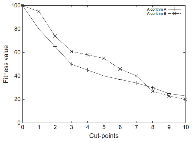
The specific number of samples and treatments to consider would depend on the characteristics of each specific situation and the available data, although a reasonable rule would be to have approximately twice the number of samples as treatments, at least (see J. Gibbons, S. Chakraborti, Nonparametric Statistical Inference, fifth ed., Chapman & Hall, 2010). Also, treatments should always be ordered in increasing order, since we are interested in analyzing the trends as the search progresses. That is, the first treatment should represent the first cut-point, the second treatment should represent the second cut-point and so on.

Under these conditions, Page’s trend test may be used to detect increasing trends in the ranks that represent the differences (or decreasing trends, if the order of the algorithms is reversed). Assuming a minimization objective, the outcome of the test can be interpreted as follows:

Significant increasing trend: If a consistently increasing trend in the ranks is found, this means that either the fitness of A is growing faster than the fitness of B or that the fitness of B is decreasing faster than the fitness of A. Since the fitness is computed as the best value found throughout the search, the former case is impossible. Hence, if an increasing trend is detected, this means that the fitness of B is decreasing faster, which means that it has a better convergence performance.
Significant decreasing trend: Following the same reasoning as above, this could only mean that the fitness of A is decreasing faster. Hence, a decreasing trend in the ranks means that A has a better convergence performance.
No significant trend: If no consistent trend is found, then nothing can be said about the relative convergence performance of two algorithms.

Alternative ranks computation procedure

Although the aforementioned procedure should be correct in most cases, it should be used with caution if any of the algorithms is unable to progress in the search for some of the functions. The most typical case of this occurring would probably be when the absolute global optimum could be reached within the evaluations limit stipulated (something that it is very likely to happen with most of the common benchmarks currently used, such as the IEEE Conference on Evolutionary Computation 2005 Special Session on Real-Parameter Optimization (P. Suganthan, N. Hansen, J. Liang, K. Deb, Y. Chen, A. Auger, S. Tiwari, Problem Definitions and Evaluation Criteria for the CEC’2005 Special Session on Real Parameter Optimization. Nanyang Technological University, Technical Report, 2005.) one). Hence, if such optimum is reached (if it is known), the computation procedure should be corrected in order rank the difference properly.

The next figure shows a graphic depicting the convergence process of two different algorithms for a given function. As can be seen, algorithm A is converging faster than algorithm B, reaching the optimum using half of the total evaluations allowed. In this situation, the test would be expected to report a positive response, showing that algorithm A has a better behavior in that problem.

However, this is not the case if the former ranking computation procedure is used. If fitness value differences between the algorithms are computed, an increasing trend would be identified from cut-points 1 to 5 (positive for algorithm A, since the differences are increasing as the algorithms proceed). However, a decreasing trend would also be detected, from cut-points 6 to 10. Clearly, this undesirable behavior is caused by the fact that the optimum has been reached too soon by algorithm A, preventing it from progressing further for the rest of the fitness evaluations.

To tackle this problem, we propose a modification to the procedure used to compute the ranks. The aim of this alternative version is to continue using the same ranking scheme as in the original approach, but fixing the ranks for those cases in which the function’s optimum is reached well before the maximum number of fitness evaluations are exhausted.

When analyzing the differences between two algorithms, A and B, as A–B, four different cases can be highlighted (by considering ranks for 10 cut-points for each case):

No algorithm reaches the optimum before the end: No further changes are necessary.
Algorithm A reaches the optimum before the end: Ranks should be modified so an increasing trend is detected from the point at which algorithm A reaches the optimum to the last cut-points of the comparison. The rest of the ranks could be assigned as above. Example: 3, 1, 2, 4, 5, 6, 7, 8, 9, 10.
Algorithm B reaches the optimum before the end: Ranks should be modified so a decreasing trend is detected from the point at which algorithm B reaches the optimum. The lowest ranks should be assigned decreasingly to the last cut-points of the comparison. The rest of the ranks could be assigned as in the first case. Example: 6, 10, 8, 9, 7, 5, 4, 3, 2, 1.
Both algorithms reach the optimum at the same cut-point: In this case, the computation of the ranks can be performed as with the original version of the test. Zero differences will be ranked using the median ranks, denoting that no trend is detected from the point in which both algorithms reached the optimum. Example: 1, 10, 9, 8, 2, 5, 5, 5, 5, 5.

As has been shown, the alternative version addresses those cases in which the global optimum is reached prior to exhausting the maximum function evaluations, preventing the algorithm from continuing with the search. In cases 2 and 3, the scheme adopted will benefit the first algorithm to converge to the optimum, and this benefit will be higher the sooner the said optimum is reached. Also, note that if case 4 is reached, the chances of not rejecting the equality hypothesis will greatly increase (as would happen naturally if the basic ranking scheme is considered).

A Case Study Analyzing some Differential Evolution Approaches.

In order to demonstrate the usefulness of the methodology proposed, the following sections will be devoted to describing a case study focused on the analysis of several Differential Evolution based techniques, and to analyzing the results obtained. Note that, even in large case studies like this one, this methodology requires to consider only a fixed number of cut-points (dependent on the number of functions considered as benchmark). This requirement is independent to other factors like population sizes or the number of iterations performed, making the test a suitable choice when analyzing complex experiments.

Functions

The study consists of 19 functions. The first six were taken from the CEC’2008 Special Session and Competition on Large Scale Global Optimization (K. Tang, X. Yao, P.N. Suganthan, C. MacNish, Y.P. Chen, C.M. Chen, Z. Yang, Benchmark Functions for the CEC’2008 Special Session and Competition on Large Scale Global Optimization. Nature Inspired Computation and Applications Laboratory, USTC, China, Technical Report, 2007). Functions F7–F11 were included as shifted versions from other common benchmarks in continuous optimization. Finally, functions F12–F19 were built for this benchmark combining two of the previous ones (at least one of the functions in each combination is non-separable). The next table shows the main characteristics of each function: Name, Range and Optimum value. The analysis of results will be carried out considering three different set-ups: 50 dimensions, 100 dimensions and 200dimensions. This will provide a clear picture on how the algorithms perform as the dimensionality of the problems increase.

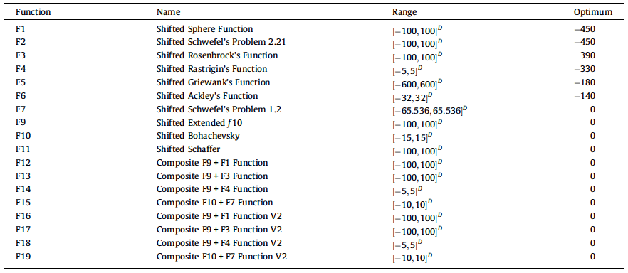
Algorithms

Six different algorithms have been chosen for this study, being all of them advanced EAs based on differential evolution:

GODE: (H. Wang, Z. Wu, S. Rahnamayan, Enhanced opposition-based differential evolution for solving high-dimensional continuous optimization problems, Soft Comput. 15 (2011) 2127–2140)
SaDE-MMTS: (S.Z. Zhao, P.N. Suganthan, S. Das, Self-adaptive differential evolution with multi-trajectory search for large scale optimization, Soft Comput. 15 (2011) 2175–2185)
SaEPSDE-MMTS: (S.Z. Zhao, P.N. Suganthan, Comprehensive comparison of convergence performance of optimization algorithms based on nonparametric statistical tests, in: Proceedings of the IEEE Congress on Evolutionary Computation, CEC 2012, Brisbane, Australia, June 10–15.)
SOUPDE: (M. Weber, F. Neri, V. Tirronen, Shuffle or update parallel differential evolution for large scale optimization, Soft Comput. 15 (2011) 2089–2107)
GADE: (Z. Yang, K. Tang, X. Yao, Scalability of generalized adaptive differential evolution for large-scale continuous optimization, Soft Comput. 15 (2011) 2141–2155)
jDElscop: (J. Brest, M.S. Maucec, Self-adaptive differential evolution algorithm using population size reduction and three strategies, Soft Comput. 15 (2011) 2157–2174)

Results and Convergence Analysis

The following three tables show a summarized version of the results obtained. Results are provided for both the original and the alternative version of the test. Each p-value of the tables is computed as the probability of rejection of the hypothesis of equality of convergence, in favor of the alternative that the method in the row converges faster than the method in the column. Rejected hypotheses (at a significance level of 0.1) are highlighted in bold.

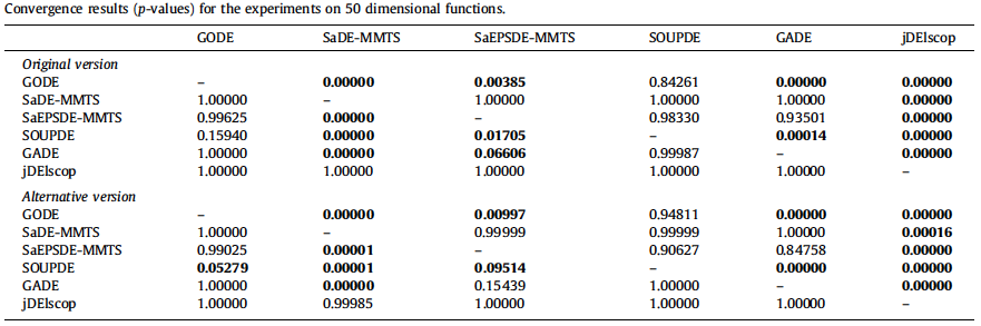
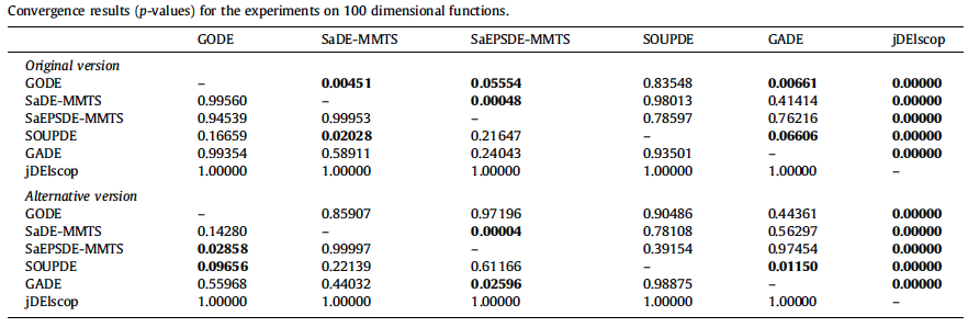
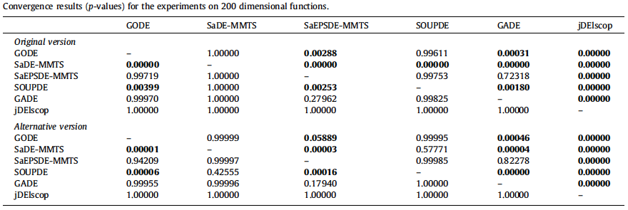
The very first fact to note here is the differences between the original and the alternative version of the test: Although in the most clear cases the results seldom change, this is not the case for some of the comparisons, for which very different p-values are obtained (particularly in the results for 100 dimensional functions).

After studying the analysis performed with the alternative version, we can draw the following conclusions:

After studying the analysis performed with the alternative version, we can draw the following conclusions:
100 dimensions: SOUPDE presents the best convergence in this scenario. GADE and SaDE-MMTS presents a better performance than SaEPSDE-MMTS, and GODE and jDElscop shows the lowest convergence speed in this case.
200 dimensions: SaDE-MMTS and SOUPDE are the best methods with respect to convergence in this case. GODE is also significantly better than SaEPSDE-MMTS and GADE, whereas jDElscop presents the worst convergence capabilities.

Although the results differ depending on the number of dimensions considered, it is safe to state that, in general, SOUPDE shows the best behavior with respect to convergence capabilities, whereas jDElscop presents the worst. A further interesting observation is in regard of the relationship between SaDE-MMTS and SaEPSDE-MMTS (the latter is better at 50 dimensions, whereas the former is at 100 dimensions and particularly at 200 dimensions).

The analysis of final results can now be refined with this convergence study. Considering both methodologies, SOUPDE shows the best performance out of the 6 differential evolution methods analyzed. The most striking difference can be found in the results of jDElscop, which has shown a marginal advantage with respect to the final results, but the worst convergence performance. This could indicate that the convergence mechanisms of jDElscop enables it to avoid local optima in a better way than the other methods, but at the cost of a low convergence speed – thus needing more functions evaluations to fully reach its best performance.

Other conclusions include the fact that, despite the similar results obtained by SaEPSDE-MMTS and SaDE-MMTS, the former should be preferred for low dimensional problems whereas SaDE-MMTS should be chosen when the number of dimensions increases. Also, GODE and GADE show a poorer performance than the rest, although the former should still be considered for low dimensional problems.

In summary, these conclusions reveal the fact that useful information about the performance of evolutionary methods in continuous optimization can be drawn if the intermediate results are analyzed. By studying convergence in depth, analyzing how the methods’ results evolve as the fitness function evaluations are consumed, new comparisons can be made depicting other useful properties of the search methods rather than just the final results at a predefined point.

Frequent Asked Questions.

What should we do if Both algorithms reach the optimum at different cut-points?: In this case, the algorithm which reached the optimum first should be preferred, i.e. follow case two if algorithm A reached it first, or case three otherwise. Note that the point of this (and the whole "alternative version") is to provide evidence that the first algorithm worked better than the second in that specific function. So that's why we only care about the algorithm which finished first, and modify the ranks accordingly.

If both algorithms reach the local optimum with the same fitness values before the end, a decreasing trend would be detected because the one algorithm converges too much? This is an alternative version for a very particular kind of problems. Ideally, to test convergence properly, algorithms should be able to progress with no limits during the time in which they are been tracked, i.e. they should be able to progress along the whole run, until the fitness allowance runs out. The alternative version tries to correct the computation in case that this property does not hold; but ideally, algorithms should never reach the optimum and thus never stop advancing in the search. If that's true, the alternative version will be equal to the regular version.

For the most problems, the algorithms both reach a position near optimum, but the error is not 0. For such case, it seems that the alternative method will not help much since I notice that in the code, 0 is used to judge if the algorithm reaches the optimum. In general, the point here is that due to precission errors it is likely that many implementations of the algorithms would not reach an error of 0, so a threshold must be selected to consider the function solved and mark that particular result as an optimum reached. At the time in which I was coding the Java program, I had no information about where to set this threshold, so I assumed that this replacement (values less than threshold ---> 0) would be applied to the input data, before applying the test (so the input data already includes those 0's). Of course, another option would be to pass this threshold as a parameter to the method, and set all the values less than threshold to 0, before carrying out the test.

Relevant Journal Papers with Data Mining and Computational Intelligence Case Studies

J. Demsar, Statistical Comparisons of Classifiers over Multiple Data Sets. Journal Of Machine Learning Research 7 (2006) 1-30 S. García, F. Herrera, An Extension on "Statistical Comparisons of Classifiers over Multiple Data Sets" for all Pairwise Comparisons. Journal of Machine Learning Research 9 (2008) 2677-2694
J. Luengo, S. García, F. Herrera, A Study on the Use of Statistical Tests for Experimentation with Neural Networks: Analysis of Parametric Test Conditions and Non-Parametric Tests. Expert Systems with Applications 36 (2009) 7798-7808 doi:10.1016/j.eswa.2008.11.041.
S. García, A. Fernández, J. Luengo, F. Herrera, A Study of Statistical Techniques and Performance Measures for Genetics-Based Machine Learning: Accuracy and Interpretability. Soft Computing 13:10 (2009) 959-977, doi:10.1007/s00500-008-0392-y.
S. García, D. Molina, M. Lozano, F. Herrera , A Study on the Use of Non-Parametric Tests for Analyzing the Evolutionary Algorithms' Behaviour: A Case Study on the CEC'2005 Special Session on Real Parameter Optimization. Journal of Heuristics, 15 (2009) 617-644. doi: 10.1007/s10732-008-9080-4.
S. García, A. Fernández, J. Luengo, F. Herrera, Advanced nonparametric tests for multiple comparisons in the design of experiments in computational intelligence and data mining: Experimental Analysis of Power. Information Sciences 180 (2010) 2044–2064. doi:10.1016/j.ins.2009.12.010.
C. Drummond , N. Japkowicz , Warning: statistical benchmarking is addictive. Kicking the habit in machine learning. Journal of Experimental & Theoretical Artificial Intelligence 22:1 (2010) 67–80 doi:10.1080/09528130903010295.
J. Derrac, S. García, D. Molina, F. Herrera, A Practical Tutorial on the Use of Nonparametric Statistical Tests as a Methodology for Comparing Evolutionary and Swarm Intelligence Algorithms. Swarm and Evolutionary Computation 1:1 (2011) 3-18. doi:10.1016/j.swevo.2011.02.002.
A. Ulas, O. T. Yildiz, E. Alpaydin , Cost-conscious comparison of supervised learning algorithms over multiple data sets. Pattern Recognition 45 (2012) 1772–1781 doi:10.1016/j.patcog.2011.10.005.
D. Berrar, J. A. Lozano, Significance tests or confidence intervals: which are preferable for the comparison of classifiers?. Journal of Experimental & Theoretical Artificial Intelligence. doi:10.1080/0952813X.2012.680252.
J. Derrac, S. García, S. Hui, P.N. Suganthan, F. Herrera, Analyzing Convergence Performance of Evolutionary Algorithms: A Statistical Approach . Information Sciences 289 (2014) 41-58. doi:10.1016/j.ins.2014.06.009.

J. Demsar, Statistical Comparisons of Classifiers over Multiple Data Sets. Journal Of Machine Learning Research 7 (2006) 1-30 link.

Abstract:While methods for comparing two learning algorithms on a single data set have been scrutinized for quite some time already, the issue of statistical tests for comparisons of more algorithms on multiple data sets, which is even more essential to typical machine learning studies, has been all but ignored. This article reviews the current practice and then theoretically and empirically examines several suitable tests. Based on that, we recommend a set of simple, yet safe and robust non-parametric tests for statistical comparisons of classifiers: the Wilcoxon signed ranks test for comparison of two classifiers and the Friedman test with the corresponding post-hoc tests for comparison of more classifiers over multiple data sets. Results of the latter can also be neatly presented with the newly introduced CD (critical difference) diagrams.

Summary:

Introduction.
Previous Work.
1. Related Theoretical Work.
2. Testing in Practice: Analysis of ICML Papers.
Statistics and Tests for Comparison of Classifiers.
1. Comparisons of Two Classifiers.
2. Comparisons of Multiple Classifiers.
Empirical Comparison of Tests.
1. Experimental Setup.
2. Comparisons of Two Classifiers.
3. Comparisons of Multiple Classifiers.
Conclusion.

S. García, F. Herrera, An Extension on "Statistical Comparisons of Classifiers over Multiple Data Sets" for all Pairwise Comparisons. Journal of Machine Learning Research 9 (2008) 2677-2694 link.

Abstract: In a recently published paper in JMLR, Demsar (2006) recommends a set of non-parametric statistical tests and procedures which can be safely used for comparing the performance of classifiers over multiple data sets. After studying the paper, we realize that the paper correctly introduces the basic procedures and some of the most advanced ones when comparing a control method. However, it does not deal with some advanced topics in depth. Regarding these topics, we focus on more powerful proposals of statistical procedures for comparing n x n classifiers. Moreover, we illustrate an easy way of obtaining adjusted and comparable p-values in multiple comparison procedures.

Summary:

Introduction.
Comparison of Multiple Classifiers: Performing All Pairwise Comparisons.
1. Advanced Procedures for Performing All Pairwise Comparisons.
2. Performing All Pairwise Comparisons: A Case Study.
Adjusted P-Values.
Experimental Framework.
Conclusions.

J. Luengo, S. García, F. Herrera , A Study on the Use of Statistical Tests for Experimentation with Neural Networks: Analysis of Parametric Test Conditions and Non-Parametric Tests. Expert Systems with Applications 36 (2009) 7798-7808 doi:10.1016/j.eswa.2008.11.041.

Abstract: In this paper, we focus on the experimental analysis on the performance in artificial neural networks with the use of statistical tests on the classification task. Particularly, we have studied whether the sample of results from multiple trials obtained by conventional artificial neural networks and support vector machines checks the necessary conditions for being analyzed through parametrical tests. The study is conducted by considering three possibilities on classification experiments: random variation in the selection of test data, the selection of training data and internal randomness in the learning algorithm. The results obtained state that the fulfillment of these conditions are problem-dependent and indefinite, which justifies the need of using non-parametric statistics in the experimental analysis.

Summary:

Introduction.
Classification algorithms and experimentation framework.
1. Artificial neural networks and support vector machines.
2. Experimentation framework
Study on the initial conditions for parametric tests using artificial neural networks
1. Conditions for the use of parametric tests.
2. Normality test over the group of data sets and algorithms.
3. Case studies of the normality property.
On the use of rank-based non-parametric tests: a short experimental study.
1. Rank-based non-parametric tests.
2. Experimental study: results and analysis.
Conclusions

S. García, A. Fernández, J. Luengo, F. Herrera, A Study of Statistical Techniques and Performance Measures for Genetics-Based Machine Learning: Accuracy and Interpretability. Soft Computing 13:10 (2009) 959-977, doi:10.1007/s00500-008-0392-y.

Abstract: The experimental analysis on the performance of a proposed method is a crucial and necessary task to carry out in a research. This paper is focused on the statistical analysis of the results in the field of genetics-based machine Learning. It presents a study involving a set of techniques which can be used for doing a rigorous comparison among algorithms, in terms of obtaining successful classification models. Two accuracy measures for multiclass problems have been employed: classification rate and Cohen’s kappa. Furthermore, two interpretability measures have been employed: size of the rule set and number of antecedents. We have studied whether the samples of results obtained by genetics-based classifiers, using the performance measures cited above, check the necessary conditions for being analysed by means of parametrical tests. The results obtained state that the fulfillment of these conditions are problem-dependent and indefinite, which supports the use of non-parametric statistics in the experimental analysis. In addition, non-parametric tests can be satisfactorily employed for comparing generic classifiers over various data-sets considering any performance measure. According to these facts, we propose the use of the most powerful non-parametric statistical tests to carry out multiple comparisons. However, the statistical analysis conducted on interpretability must be carefully considered.

Summary:

Introduction.
Genetics-based machine learning algorithms for classification.
Performance measures and experimental results.
1. Accuracy measures for multi-class problems.
2. Interpretability measures.
3. Experimental results.
Study on the initial conditions for parametric tests using genetics-based machine learning.
1. Conditions for a safe use of parametric tests.
2. Analysis of the conditions for a safe use of parametric tests.
3. Case studies of the normality property.
Non-parametric tests for comparing two algorithms in multiple data-set analysis.
1. Wilcoxon signed-ranks test.
2. A case study in GBML: performing pairwise comparisons.
Non-parametric tests for multiple comparisons among more than two algorithms.
1. Friedman test and post-hoc tests.
2. A case study in GBML: performing multiple comparisons.
Analysing interpretability of models.
Conclusions.

S. García, D. Molina, M. Lozano, F. Herrera, A Study on the Use of Non-Parametric Tests for Analyzing the Evolutionary Algorithms' Behaviour: A Case Study on the CEC'2005 Special Session on Real Parameter Optimization. Journal of Heuristics, 15 (2009) 617-64 doi: 10.1007/s10732-008-9080-4.

Abstract: In recent years, there has been a growing interest for the experimental analysis in the field of evolutionary algorithms. It is noticeable due to the existence of numerous papers which analyze and propose different types of problems, such as the basis for experimental comparisons of algorithms, proposals of different methodologies in comparison or proposals of use of different statistical techniques in algorithms’ comparison.
In this paper, we focus our study on the use of statistical techniques in the analysis of evolutionary algorithms’ behaviour over optimization problems. A study about the required conditions for statistical analysis of the results is presented by using some models of evolutionary algorithms for real-coding optimization. This study is conducted in two ways: single-problem analysis and multiple-problem analysis. The results obtained state that a parametric statistical analysis could not be appropriate specially when we deal with multiple-problem results. In multiple-problem analysis, we propose the use of non-parametric statistical tests given that they are less restrictive than parametric ones and they can be used over small size samples of results. As a case study, we analyze the published results for the algorithms presented in the CEC’2005 Special Session on Real Parameter Optimization by using non-parametric test procedures.

Summary:

Introduction.
Preliminaries: settings of the CEC’2005 Special Session.
1. Evolutionary algorithms.
2. Test functions.
3. Characteristics of the experimentation.
Study of the required conditions for the safe use of parametric tests.
1. Conditions for the safe use of parametric tests.
2. On the study of the required conditions over single-problem analysis.
3. On the study of the required conditions over multiple-problem analysis.
A case study: on the use of non-parametric statistics for comparing the results of the CEC’2005 Special Session in Real Parameter Optimization.
Some considerations on the use of non-parametric tests.
Conclusions

S. García, A. Fernández, J. Luengo, F. Herrera, Advanced nonparametric tests for multiple comparisons in the design of experiments in computational intelligence and data mining: Experimental Analysis of Power. Information Sciences 180 (2010) 2044–206 doi:10.1016/j.ins.2009.1010.

Abstract: Experimental analysis of the performance of a proposed method is a crucial and necessary task in an investigation. In this paper, we focus on the use of nonparametric statistical inference for analyzing the results obtained in an experiment design in the field of computational intelligence. We present a case study which involves a set of techniques in classification tasks and we study a set of nonparametric procedures useful to analyze the behavior of a method with respect to a set of algorithms, such as the framework in which a new proposal is developed.

Particularly, we discuss some basic and advanced nonparametric approaches which improve the results offered by the Friedman test in some circumstances. A set of post hoc procedures for multiple comparisons is presented together with the computation of adjusted p-values. We also perform an experimental analysis for comparing their power, with the objective of detecting the advantages and disadvantages of the statistical tests described. We found that some aspects such as the number of algorithms, number of data sets and differences in performance offered by the control method are very influential in the statistical tests studied. Our final goal is to offer a complete guideline for the use of nonparametric statistical procedures for performing multiple comparisons in experimental studies.

Summary:

Introduction.
Experimental Framework.
Basic nonparametric tests for performing multiple comparisons: Friedman test, Multiple Sign-test and Contrast Estimation based on medians.
1. Friedman test and Iman-Davenpor extension.
2. Multiple Sign-Test.
3. Constrast Estimation based on medians.
Advanced nonparametric tests for performing multiple comparisons: Friedman Aligned Ranks and the test of Quade.
1. Friedman Aligned Ranks.
2. Quade Test.
A candidate set of post hoc tests: p-values and adjusted p-values.
1. Post hoc procedures.
2. Experimental Study.
Experimental analysis: power of the multiple comparisons tests.
1. Analysis of the power of nonparametric multiple comparisons tests.
2. Analysis of the power of the post hoc procedures.
3. Analysis of the stability of the Quade test.
Summary and suggestions.
Conclusions

C. Drummond , N. Japkowicz, Warning: statistical benchmarking is addictive. Kicking the habit in machine learning. Journal of Experimental & Theoretical Artificial Intelligence 22:1 (2010) 67–80 doi:10.1080/09528130903010295.

Abstract: Algorithm performance evaluation is so entrenched in the machine learning community that one could call it an addiction. Like most addictions, it is harmful and very difficult to give up. It is harmful because it has serious limitations. Yet, we have great faith in practicing it in a ritualistic manner: we follow a fixed set of rules telling us the measure, the data sets and the statistical test to use. When we read a paper, even as reviewers, we are not sufficiently critical of results that follow these rules. Here, we will debate what are the limitations and how to best address them. This article may not cure the addiction but hopefully it will be a good first step along that road.

Summary:

Introduction.
What is wrong with what we are doing now?.
1. What are we measuring?.
2. What does a statistical test buy us?.
3. What do our data sets represent?.
What is the alternative?.
1. What should we measure?.
2. What tests should we do?.
3. What data should we use?.
Conclusions.

J. Derrac, S. García, D. Molina,F. Herrera, A Practical Tutorial on the Use of Nonparametric Statistical Tests as a Methodology for Comparing Evolutionary and Swarm Intelligence Algorithms. Swarm and Evolutionary Computation 1:1 (2011) 3-18. doi:10.1016/j.swevo.2011.0002.

Abstract: The interest in nonparametric statistical analysis has grown recently in the field of computational intelligence. In many experimental studies, the lack of the required properties for a proper application of parametric procedures – independence, normality, and homoscedasticity – yields to nonparametric ones the task of performing a rigorous comparison among algorithms.

In this paper, we will discuss the basics and give a survey of a complete set of nonparametric procedures developed to perform both pairwise and multiple comparisons, for multi-problem analysis. The test problems of the CEC’2005 special session on real parameter optimization will help to illustrate the use of the tests throughout this tutorial, analyzing the results of a set of well-known evolutionary and swarm intelligence algorithms. This tutorial is concluded with a compilation of considerations and recommendations, which will guide practitioners when using these tests to contrast their experimental results.

Summary:

Introduction.
Preliminaries.
1. Benchmark functions: CEC’2005 special session on real parameter optimization.
2. Evolutionary and swarm intelligence algorithms.
3. Some basic concepts on inferential statistics.
Pairwise comparisons.
1. A simple first-sight procedure: the Sign test.
2. The Wilcoxon signed ranks test.
Multiple comparisons with a control method.
1. Multiple Sign test.
2. The Friedman, Friedman Aligned Ranks, and Quade tests.
3. Post-hoc procedures.
4. Contrast Estimation.
Multiple comparisons among all methods.
Considerations and recommendations on the use of nonparametric tests.
1. General considerations.
2. Multiple comparisons with a control method.
3. Multiple comparisons among all methods.
Conclusions

A. Ulas, O. T. Yildiz, E. Alpaydin , Cost-conscious comparison of supervised learning algorithms over multiple data sets. Pattern Recognition 45 (2012) 1772–1781 doi:10.1016/j.patcog.2011.10.005.

Abstract: In the literature,there exist statistical tests to compare supervised learning algorithms on multiple data sets in terms of accuracy but they do not always generate an ordering. We propose Multi2Test, a generalization of our previous work,for ordering multiple learning algorithms on multiple data sets from ‘‘best’’ to ‘‘worst’’ where our goodness measure is composed of a prior cost term additional to generalization error. Our simulations show that Multi2Test generates orderings using pairwise tests on error and different types of cost using time and space complexity of the learning algorithms.

Summary:

Introduction.
Comparing multiple algorithms over multiple datasets.
1. The sign test.
2. Multiple pairwise comparisons on multiple datasets.
3. Correction for multiple comparisons.
Multi2Test.
1. MultiTest.
2. Multi2Test.
Results.
1. Experimental setup.
2. The sign test over averages.
3. Friedman’s test and Bergmann-Hommel’s dynamic procedure.
4. The sign test over pair wise tests.
5. Applying Multi2Test.
  1. Training time as cost.
  2. Space complexity as cost.
6. Testing MultiTest and Multi2Test.
7. Verification of results on test.
Discussions and conclusions.

D. Berrar, J. A. Lozano , Significance tests or confidence intervals: which are preferable for the comparison of classifiers?. Journal of Experimental & Theoretical Artificial Intelligence, In press (2012) doi:10.1080/0952813X.201680252.

Abstract: Null hypothesis significance tests and their p-values currently dominate the statistical evaluation of classifiers in machine learning. Here, we discuss fundamental problems of this research practice. We focus on the problem of comparing multiple fully specified classifiers on a small-sample test set. On the basis of the method by Quesenberry and Hurst, we derive confidence intervals for the effect size, i.e. the difference in true classification performance. These confidence intervals disentangle the effect size from its uncertainty and thereby provide information beyond the p-value. This additional information can drastically change the way in which classification results are currently interpreted, published and acted upon. We illustrate how our reasoning can change, depending on whether we focus on p-values or confidence intervals. We argue that the conclusions from comparative classification studies should be based primarily on effect size estimation with confidence intervals, and not on significance tests and p-values.

Summary:

Introduction.
Problem statement.
Significance tests and CIs: two sides of the same coin?.
Formal preliminaries.
Significance test for the difference in performance on the same test set and a 0-1 loss function.
CIs for the effect size.
Materials and methods.
Results.
9. Discussion and conclusions.

J. Derrac, S. García, S. Hui, P.N. Suganthan, F. Herrera, Analyzing Convergence Performance of Evolutionary Algorithms: A Statistical Approach. Information Sciences 289 (2014) 41-58. doi:10.1016/j.ins.2010009.

Abstract: The analysis of the performance of different approaches is a staple concern in the design of Computational Intelligence experiments. Any proper analysis of evolutionary optimization algorithms should incorporate a full set of benchmark problems and state-of-the-art comparison algorithms. For the sake of rigor, such an analysis may be completed with the use of statistical procedures, supporting the conclusions drawn. In this paper, we point out that these conclusions are usually limited to the final results, whereas intermediate results are seldom considered. We propose a new methodology for comparing evolutionary algorithms’ convergence capabilities, based on the use of Page’s trend test. The methodology is presented with a case of use, incorporating real results from selected techniques of a recent special issue. The possible applications of the method are highlighted, particularly in those cases in which the final results do not enable a clear evaluation of the differences among several evolutionary techniques.

Summary:

Introduction.
Background.
1. Nonparametric tests.
2. Page's trend test.
Using Page’s trend test for convergence analysis.
1. Using Page’s trend test.
2. Alternative ranks computation procedure.
Case of use: On analyzing the performance of several Differential Evolution based approaches.
1. Functions.
2. Algorithms considered.
Results and analysis.
1. Final results analysis: Friedman and Bergmann tests.
2. Convergence analysis.
Conclusions.

Relevant books on Non-parametric tests

The reader can increase the information provided in this web page. We recommend the reading of the following books:

	D.J. Sheskin. Handbook of Parametric and Non-Parametric Statistical Procedures. CRC Press (2007)
	J.H. Zar. Biostatistical Analysis. Prentice Hall. (2009)
	W.W. Daniel. Applied Nonparametric Statistics. Houghton Mifflin Harcourt. (1990)
	W.J. Conover. Practical Nonparametric Statistics. Wiley. (1998)
	M. Hollander and D.A. Wolfe. Nonparametric Statistical Methods.Wiley-Interscience. (1999)
	J.J. Higgins. Introduction to Modern Nonparametric Statistics. Duxbury Press. (2003).

Topic Slides

S. García, F. Herrera (November 2010) . How must I conduct statistical comparisons in my Experimental Study? Design of Experiments in Data Mining/Computational Intelligence. On the use Non-parametric Statistical Tests. Some Cases of Study.

H. Takagi (April 2013) . Statistical Tests for Computational Intelligence Research and Human Subjective Tests. 2013 IEEE Symposium Series on Computational Intelligence. http://www.design.kyushu-u.ac.jp/~takagi/TAKAGI/StatisticalTests.html

Software and User's Guide

We offer a software developed in JAVA which calculates all the multiple comparisons procedures described in this web page. It allows as input files in CSV format and obtains as output a LaTeX file with tabulated information about Friedman, Iman-Davenport, Friedman Aligned Ranks, Quade, Contrast Estimation, Bonferroni-Dunn, Holm, Hochberg, Hommel, Holland, Rom, Finner, Li, Shaffer and Bergamnn-Hommel tests. It also computes and shows the adjusted p-values.

The software for computing the advanced multiple comparison procedures described in (S. García, A. Fernández, J. Luengo, F. Herrera, Advanced nonparametric tests for multiple comparisons in the design of experiments in computational intelligence and data mining: Experimental Analysis of Power. Information Sciences 180 (2010) 2044–2064. doi:10.1016/j.ins.2009.12.010.) can be found in CONTROLTEST package.

The software for conducting multiple comparison involving all possible pairwise comparisons described in (S. García, F. Herrera, An Extension on "Statistical Comparisons of Classifiers over Multiple Data Sets" for all Pairwise Comparisons. Journal of Machine Learning Research 9 (2008) 2677-2694) can be found in MULTIPLETEST package.

The first one (CONTROLTEST package) can be used to:

Read data of results of k algorithms over N case problems in CSV format. The data can correspond to accuracy, AUC or any other performance measure.
Compute the rankings through the Friedman Aligned Ranks and Quade procedures of k algorithms over N case problems.
Compute the Friedman and Iman-Davenport, Friedman Aligned-Ranks and Quade Statistics corresponding to the input data.
Show the tables with the set of hypotheses, unadjusted p-values for each comparison and adjusted level of significance for Bonferroni-Dunn, Holm and Hochberg, Hommel, Holland, Rom, Finner and Liprocedures: 1 x n comparison.
Show the table with adjusted p-values for the procedures 1 x n mentioned in the previous item.
Give a report detailing the rejected hypotheses considering the levels of significance α = 0.05 and α = 0.10.

The second one (MULTIPLETEST package) can be used to:

Read data of results of k algorithms over N case problems in CSV format. The data can correspond to accuracy, AUC or any other performance measure.
Compute the Friedman and Iman-Davenport, Statistics corresponding to the input data.
Show the tables with the set of hypotheses, unadjusted p-values for each comparison and adjusted level of significance for Bonferroni-Dunn, Holm and Hochberg: 1 x n comparison
Show the table with adjusted p-values for the procedures 1 x n mentioned in the previous item.
Show the tables with the set of hypotheses, unadjusted p-values for each comparison and adjusted level of significance for Nemenyi, Holm, Shaffer's static and Bergmann-Hommel's dynamic procedures: n x n comparison.
Show the table with adjusted p-values for the procedures n x n mentioned in the previous item.
Give a report detailing the rejected hypotheses considering the levels of significance α = 0.05 and α = 0.10.

The programs are written in JAVA, so an installed JVM in the computer is needed in order to run it. To do this, execute:
java Friedman < data file >
An example of data is included in the package. The output is given in LATEX format on standard output. We recommend to redirect the output to a file in the following manner:
java Friedman data.csv > output.tex

The software for analyzing the convergence performance of evolutionary algorithms through the Page test is describen in (J. Derrac, S. García, S. Hui, P.N. Suganthan, F. Herrera, Analyzing Convergence Performance of Evolutionary Algorithms: A Statistical Approach. Information Sciences 289 (2014) 41-58. doi:10.1016/j.ins.2014.06.009

The Java package (Page Test package) can be downloaded.

You are here

Statistical Inference in Computational Intelligence and Data Mining

Introduction to Inferential Statistics

Conditions for the safe use of Nonparametric Tests

Nonparametric Tests

Pairwise comparisons

Multiple comparisons with a control method

Post-hoc Procedures

Adjusted p-values

Multiple comparisons among all methods

Case Studies

Multiple comparisons with a control method.

Multiple comparisons among all methods.

Considerations and Recommendations on the Use of Nonparametric Tests

Considerations on the use of Nonparametric Tests.

Pairwise comparisons.

Multiple Comparisons with a control method.

Recommendations on the use of Nonparametric Tests

Pairwise comparisons.

Multiple comparisons with a control method.

Multiple comparisons among all methods.

Statistical Analysis of Convergence Performance of Evolutionary Algorithms

Background to the Analysis of Convergence in Evolutionary Algorithms.

Page's Trend Test.

Usage of the Page Test for Convergence Analysis.

A Case Study Analyzing some Differential Evolution Approaches.

Frequent Asked Questions.

Relevant Journal Papers with Data Mining and Computational Intelligence Case Studies

Relevant books on Non-parametric tests

Topic Slides

Software and User's Guide

User login

SCI2S Web-site Related