
Integrating Instance Selection, Instance Weighting and Feature Weighting for Nearest Neighbor Classifiers by Co-evolutionary Algorithms - Complementary Material
This Website contains complementary material to the paper:
J. Derrac, I.Triguero, S. García and F.Herrera, Integrating Instance Selection, Instance Weighting and Feature Weighting for Nearest Neighbor Classifiers by Co-evolutionary Algorithms. IEEE Transactions on Systems, Man, and Cybernetics, Part B: Cybernetics 42:5 (2012) 1383-1397, doi: 10.1109/TSMCB.2012.2191953 ![]()
The web is organized according to the following summary:
Results
Standard results
In this section, we report the full results obtained in the experimental study. For each pair data set/algorithm, we report its average performance results (using accuracy, kappa, reduction rate and/or time elapsed) and standard deviations. Furthermore, we also provide graphics depicting the more relevant results achieved, and the results of the statistical comparisons performed. The results shown in all the tables can be downloaded as an Excel document by clicking on the following link: ![]()
Comparison between CIW-NN and evolutionary proposals for k-NN based classification
This subsection shows the results achieved in the experimental comparison performed between CIW-NN and evolutionary proposals for k-NN based classification. The tables shown here can be also downloaded as an Excel document by clicking on the following link: ![]()
Tables 4 and 5 shows average accuracy and kappa results, respectively, achieved in training and test phases. Table 6 shows the average time elapsed and reduction rates.
Table 4. Accuracy results of the comparison between CIW-NN and its basic components.
| CIW-NN | IS-CHC | SSGA-FW | SSGA-IW | SSMA | 1-NN | |||||||||||||||||||
|---|---|---|---|---|---|---|---|---|---|---|---|---|---|---|---|---|---|---|---|---|---|---|---|---|
| Training | Test | Training | Test | Training | Test | Training | Test | Training | Test | Training | Test | |||||||||||||
| Data set | Acc. | Std. | Acc. | Std. | Acc. | Std. | Acc. | Std. | Acc. | Std. | Acc. | Std. | Acc. | Std. | Acc. | Std. | Acc. | Std. | Acc. | Std. | Acc. | Std. | Acc. | Std. |
| Australian | 85.52 | 1.05 | 81.74 | 3.44 | 86.44 | 0.33 | 81.45 | 4.29 | 83.95 | 0.88 | 81.01 | 5.63 | 81.51 | 0.80 | 80.87 | 3.42 | 88.55 | 0.35 | 85.51 | 3.49 | 80.71 | 0.84 | 81.45 | 4.29 |
| Balance | 83.64 | 1.05 | 85.75 | 4.13 | 86.54 | 0.97 | 79.04 | 6.46 | 77.65 | 0.71 | 73.76 | 3.99 | 82.33 | 0.58 | 80.33 | 3.96 | 90.77 | 0.46 | 88.32 | 3.12 | 78.95 | 0.87 | 79.04 | 6.46 |
| Bands | 71.14 | 1.82 | 75.52 | 5.57 | 72.60 | 1.39 | 74.04 | 6.58 | 80.85 | 1.16 | 72.75 | 5.86 | 74.79 | 1.07 | 72.92 | 6.90 | 78.97 | 1.4 | 62.34 | 3.06 | 73.47 | 1.28 | 74.04 | 6.58 |
| Breast | 76.30 | 1.57 | 70.62 | 7.44 | 76.15 | 1.10 | 66.04 | 6.92 | 72.45 | 1.53 | 63.06 | 9.27 | 73.23 | 0.73 | 69.98 | 6.38 | 78.17 | 1.03 | 71.42 | 5.86 | 65.11 | 1.39 | 65.35 | 6.07 |
| Bupa | 71.57 | 2.79 | 60.95 | 7.50 | 69.92 | 2.57 | 62.51 | 7.38 | 70.04 | 1.75 | 62.91 | 6.67 | 63.70 | 1.23 | 62.29 | 6.57 | 77.58 | 1.4 | 62.17 | 6.26 | 61.22 | 1.37 | 61.08 | 6.88 |
| Car | 88.58 | 2.01 | 95.89 | 1.17 | 86.05 | 1.10 | 85.65 | 1.81 | 95.18 | 0.22 | 94.91 | 1.24 | 87.18 | 0.26 | 86.34 | 2.14 | 95.29 | 0.99 | 92.31 | 3.36 | 86.09 | 0.28 | 85.65 | 1.81 |
| Cleveland | 61.64 | 1.85 | 56.43 | 5.54 | 61.39 | 1.19 | 53.14 | 7.45 | 59.77 | 1.46 | 52.48 | 5.06 | 60.43 | 0.72 | 56.45 | 6.30 | 63.99 | 1.37 | 56.12 | 9.05 | 52.77 | 0.96 | 53.14 | 7.45 |
| Contraceptive | 48.04 | 1.28 | 45.22 | 2.59 | 48.95 | 0.53 | 42.63 | 3.54 | 47.70 | 1.02 | 44.06 | 4.61 | 45.86 | 0.52 | 44.61 | 2.99 | 58.6 | 1.2 | 47.73 | 4.39 | 42.97 | 0.87 | 42.77 | 3.69 |
| Dermatology | 96.02 | 1.50 | 96.72 | 3.17 | 96.87 | 0.51 | 95.35 | 3.45 | 99.00 | 0.36 | 96.45 | 2.98 | 94.41 | 1.85 | 94.26 | 4.60 | 97.75 | 0.45 | 94.02 | 3.96 | 95.63 | 0.59 | 95.35 | 3.45 |
| German | 72.16 | 1.25 | 72.10 | 2.51 | 73.38 | 0.55 | 70.50 | 4.25 | 75.03 | 0.71 | 69.50 | 3.35 | 72.26 | 0.62 | 71.90 | 3.73 | 81.11 | 0.79 | 71.2 | 2.71 | 68.97 | 0.76 | 70.50 | 4.25 |
| Glass | 68.91 | 1.93 | 75.72 | 11.13 | 73.22 | 1.46 | 74.50 | 12.50 | 80.74 | 2.47 | 72.36 | 10.71 | 71.49 | 1.73 | 69.35 | 10.03 | 75.19 | 1.38 | 70.13 | 13.18 | 70.77 | 1.86 | 73.61 | 11.91 |
| Hayes-roth | 78.11 | 1.62 | 72.15 | 12.73 | 70.88 | 4.72 | 71.01 | 10.26 | 78.02 | 0.84 | 69.96 | 11.79 | 79.12 | 1.09 | 73.03 | 11.56 | 67.01 | 1.95 | 62.33 | 11.76 | 35.44 | 1.60 | 35.70 | 9.11 |
| Housevotes | 96.02 | 1.12 | 94.93 | 4.12 | 94.99 | 0.59 | 91.24 | 6.02 | 96.25 | 0.71 | 93.78 | 3.29 | 91.77 | 0.96 | 91.23 | 5.29 | 96.09 | 0.95 | 93.54 | 5.97 | 91.83 | 0.82 | 91.24 | 6.11 |
| Iris | 96.00 | 0.82 | 93.33 | 5.96 | 97.93 | 0.65 | 93.33 | 5.16 | 97.26 | 0.47 | 94.00 | 4.67 | 96.89 | 0.55 | 94.00 | 5.54 | 98.22 | 0.76 | 94 | 3.59 | 95.48 | 0.52 | 93.33 | 5.16 |
| Lymphography | 85.67 | 2.44 | 79.30 | 12.22 | 87.17 | 2.48 | 73.87 | 8.77 | 87.92 | 1.70 | 76.54 | 6.13 | 79.66 | 0.94 | 77.34 | 12.08 | 87.54 | 1.87 | 75.85 | 14.15 | 74.63 | 1.76 | 73.87 | 8.77 |
| Monk-2 | 88.45 | 2.08 | 100.00 | 0.00 | 87.58 | 1.47 | 95.32 | 5.42 | 100.00 | 0.00 | 100.00 | 0.00 | 74.72 | 1.09 | 75.09 | 3.80 | 96.37 | 0.84 | 96.81 | 2.73 | 77.55 | 1.09 | 77.91 | 5.42 |
| Movement | 61.48 | 1.37 | 83.06 | 3.32 | 96.64 | 0.47 | 86.39 | 2.26 | 98.29 | 0.62 | 86.67 | 2.83 | 97.16 | 0.34 | 88.06 | 4.34 | 86.04 | 0.57 | 85.04 | 5.46 | 81.48 | 0.63 | 81.94 | 2.26 |
| New Thyroid | 96.13 | 1.53 | 95.82 | 3.15 | 70.96 | 1.13 | 97.23 | 3.52 | 87.53 | 0.69 | 96.28 | 3.79 | 88.61 | 1.16 | 95.84 | 4.81 | 97.62 | 0.7 | 95.87 | 4.34 | 96.64 | 1.13 | 97.23 | 3.52 |
| Pima | 72.82 | 1.01 | 71.24 | 2.03 | 76.88 | 0.75 | 70.33 | 3.99 | 73.50 | 1.01 | 70.71 | 3.72 | 71.25 | 0.45 | 70.59 | 3.03 | 82.31 | 0.84 | 72.54 | 4.09 | 70.53 | 0.87 | 70.33 | 3.99 |
| Saheart | 73.38 | 1.57 | 65.37 | 5.33 | 74.53 | 2.05 | 64.49 | 7.51 | 69.34 | 0.83 | 64.06 | 8.74 | 66.21 | 1.05 | 64.28 | 6.71 | 78.19 | 1.21 | 70.56 | 4.59 | 64.55 | 1.08 | 64.49 | 7.51 |
| Sonar | 79.91 | 2.87 | 87.00 | 3.38 | 84.88 | 2.64 | 85.55 | 6.55 | 93.86 | 1.64 | 85.07 | 7.72 | 88.46 | 0.15 | 86.02 | 1.37 | 88.57 | 1.45 | 78.33 | 8.64 | 86.32 | 1.66 | 85.55 | 6.55 |
| Spectfheart | 82.98 | 2.84 | 77.92 | 13.60 | 83.15 | 1.27 | 69.70 | 14.94 | 82.65 | 3.16 | 74.63 | 14.17 | 79.48 | 3.05 | 78.68 | 13.48 | 85.31 | 1.31 | 78.7 | 6.81 | 69.46 | 3.13 | 69.70 | 8.43 |
| Tae | 55.19 | 0.91 | 65.71 | 3.26 | 61.44 | 1.25 | 65.04 | 2.56 | 69.54 | 0.79 | 68.38 | 2.10 | 67.41 | 0.57 | 63.04 | 2.56 | 60.12 | 2.4 | 53.17 | 14.92 | 42.10 | 0.57 | 40.50 | 2.56 |
| Tic-tac-toe | 75.84 | 2.06 | 87.37 | 3.34 | 76.51 | 1.18 | 82.07 | 5.60 | 92.59 | 0.96 | 91.33 | 4.21 | 73.13 | 1.54 | 73.07 | 2.96 | 85.5 | 1.76 | 73.91 | 3.55 | 73.13 | 1.13 | 73.07 | 5.60 |
| Vehicle | 66.07 | 1.12 | 71.28 | 0.79 | 67.76 | 0.99 | 70.10 | 0.81 | 74.97 | 0.14 | 71.16 | 0.65 | 68.99 | 0.97 | 66.55 | 1.37 | 77.06 | 0.93 | 64.3 | 5.1 | 69.40 | 0.22 | 70.10 | 0.81 |
| Vowel | 72.44 | 0.84 | 98.28 | 3.78 | 77.51 | 0.74 | 99.39 | 4.85 | 99.61 | 0.39 | 99.29 | 2.75 | 98.96 | 0.50 | 98.38 | 2.76 | 85.52 | 0.81 | 84.95 | 3.71 | 99.07 | 0.76 | 99.39 | 4.85 |
| Wine | 97.50 | 0.60 | 97.16 | 2.46 | 98.32 | 0.36 | 95.52 | 2.59 | 99.38 | 0.44 | 96.63 | 3.16 | 99.06 | 0.30 | 97.75 | 1.60 | 98.88 | 0.73 | 95.52 | 5.45 | 95.57 | 0.34 | 95.52 | 2.59 |
| Wisconsin | 96.71 | 1.43 | 96.00 | 2.84 | 97.09 | 0.60 | 95.57 | 4.17 | 97.82 | 0.75 | 95.57 | 3.53 | 96.96 | 0.86 | 96.42 | 3.44 | 97.68 | 0.31 | 96.42 | 2.5 | 95.69 | 0.66 | 95.57 | 3.91 |
| Yeast | 52.17 | 2.84 | 52.76 | 3.89 | 56.40 | 1.88 | 52.23 | 4.97 | 55.32 | 0.53 | 50.81 | 4.97 | 55.26 | 1.54 | 52.63 | 5.55 | 66.08 | 0.73 | 56.54 | 4.55 | 50.78 | 0.75 | 50.47 | 6.57 |
| Zoo | 90.69 | 2.04 | 97.50 | 3.61 | 94.26 | 2.12 | 96.83 | 4.72 | 99.35 | 1.03 | 96.83 | 4.94 | 97.12 | 0.97 | 95.58 | 4.13 | 91.92 | 3.77 | 93.5 | 7.24 | 92.08 | 1.16 | 92.81 | 4.35 |
| Average | 78.04 | 1.64 | 80.09 | 4.80 | 79.55 | 1.30 | 78.00 | 5.64 | 83.18 | 0.97 | 78.83 | 5.08 | 79.25 | 0.94 | 77.56 | 5.11 | 83.73 | 1.16 | 77.44 | 5.92 | 74.61 | 1.03 | 74.69 | 5.36 |
Table 5. Kappa results of the comparison between CIW-NN and its basic components.
| CIW-NN | IS-CHC | FW-SSGA | IW-SSGA | SSMA | 1-NN | |||||||||||||||||||
|---|---|---|---|---|---|---|---|---|---|---|---|---|---|---|---|---|---|---|---|---|---|---|---|---|
| Training | Test | Training | Test | Training | Test | Training | Test | Training | Test | Training | Test | |||||||||||||
| Data set | Kap. | Std. | Kap. | Std. | Kap. | Std. | Kap. | Std. | Kap. | Std. | Kap. | Std. | Kap. | Std. | Kap. | Std. | Kap. | Std. | Kap. | Std. | Kap. | Std. | Kap. | Std. |
| Australian | .7084 | .0223 | .6304 | .0855 | .7267 | .0223 | .6248 | .1073 | .6752 | .0178 | .6167 | .0858 | .6272 | .0166 | .6137 | .0872 | .7685 | .0072 | .7062 | .0723 | .6100 | .0179 | .6248 | .0902 |
| Balance | .6972 | .0167 | .7357 | .1004 | .7504 | .0167 | .6351 | .1110 | .6067 | .0132 | .5461 | .1004 | .6722 | .0141 | .6357 | .1077 | .8289 | .0085 | .7834 | .0575 | .6308 | .0145 | .6351 | .1086 |
| Bands | .3734 | .0277 | .4847 | .1386 | .4014 | .0277 | .4677 | .1392 | .6062 | .0252 | .4440 | .1381 | .4711 | .0255 | .4316 | .1379 | .5522 | .0325 | .1762 | .0637 | .4550 | .0272 | .4677 | .1398 |
| Breast | .3134 | .0502 | .2006 | .1693 | .3327 | .0502 | .1765 | .1831 | .3328 | .0392 | .1376 | .1700 | .1983 | .0393 | .1236 | .1711 | .405 | .0384 | .2123 | .1516 | .1229 | .0395 | .1137 | .1826 |
| Bupa | .3277 | .0355 | .1629 | .1475 | .3615 | .0355 | .2291 | .1758 | .3819 | .0285 | .2415 | .1376 | .2252 | .0272 | .1962 | .1463 | .5284 | .0302 | .2131 | .1149 | .1998 | .0295 | .1953 | .1479 |
| Car | .7475 | .0085 | .9109 | .0458 | .6909 | .0085 | .6538 | .0459 | .8942 | .0072 | .8881 | .0482 | .7365 | .0070 | .7206 | .0454 | .8964 | .0221 | .8353 | .0692 | .6647 | .0077 | .6538 | .0495 |
| Cleveland | .3466 | .0188 | .2672 | .1177 | .3423 | .0188 | .2730 | .1171 | .3623 | .0162 | .2585 | .1099 | .2853 | .0168 | .2237 | .1083 | .394 | .0291 | .2789 | .1108 | .2607 | .0176 | .2730 | .1196 |
| Contraceptive | .1598 | .0146 | .1202 | .0625 | .2063 | .0146 | .1163 | .0679 | .1926 | .0125 | .1394 | .0600 | .1145 | .0131 | .0948 | .0565 | .3515 | .0213 | .1845 | .0708 | .1236 | .0133 | .1199 | .0625 |
| Dermatology | .9502 | .0078 | .9588 | .0424 | .9609 | .0078 | .9418 | .0511 | .9875 | .0070 | .9555 | .0442 | .9302 | .0072 | .9282 | .0431 | .9719 | .0057 | .925 | .0498 | .9453 | .0078 | .9418 | .0457 |
| German | .3943 | .0176 | .2712 | .0940 | .2247 | .0176 | .2800 | .0925 | .3884 | .0148 | .2519 | .0959 | .2237 | .0154 | .2131 | .0898 | .5034 | .028 | .2422 | .0789 | .2482 | .0159 | .2800 | .0980 |
| Glass | .5564 | .0338 | .6640 | .1584 | .6274 | .0338 | .6529 | .1917 | .7384 | .0266 | .6219 | .1511 | .6004 | .0258 | .5721 | .1598 | .6552 | .0185 | .589 | .176 | .6043 | .0269 | .6415 | .1677 |
| Hayes-roth | .6657 | .0380 | .5587 | .1815 | .5544 | .0380 | .5244 | .1797 | .6585 | .0325 | .4946 | .1847 | .6792 | .0293 | .5761 | .1766 | .4936 | .0309 | .4049 | .1921 | -.0124 | .0325 | .0103 | .1868 |
| Housevotes | .9166 | .0226 | .8930 | .1314 | .8948 | .0226 | .8172 | .1406 | .9209 | .0174 | .8693 | .1314 | .8283 | .0178 | .8187 | .1312 | .9175 | .0208 | .8634 | .1267 | .8290 | .0179 | .8181 | .1324 |
| Iris | .9400 | .0104 | .9000 | .0750 | .9689 | .0104 | .9000 | .0903 | .9589 | .0080 | .9100 | .0770 | .9533 | .0081 | .9100 | .0737 | .9733 | .0113 | .91 | .0539 | .9322 | .0082 | .9000 | .0816 |
| Lymphography | .7165 | .0474 | .5944 | .1728 | .7470 | .0474 | .4889 | .2048 | .7677 | .0358 | .5421 | .1775 | .5994 | .0349 | .5479 | .1758 | .7591 | .035 | .5332 | .2659 | .5121 | .0364 | .4889 | .1882 |
| Monk-2 | .7688 | .0248 | 1.0 | .0000 | .7507 | .0248 | .7546 | .1355 | 1.0 | .0000 | 1.0 | .0000 | .4831 | .0228 | .4874 | .1126 | .9274 | .0168 | .9359 | .0541 | .5424 | .0238 | .5474 | .1167 |
| Movement | .5873 | .0165 | .8180 | .0478 | .6888 | .0165 | .8537 | .0548 | .8664 | .0118 | .8567 | .0488 | .8780 | .0131 | .8716 | .0458 | .8332 | .0154 | .8380 | .0356 | .8016 | .0131 | .8060 | .0490 |
| New Thyroid | .9147 | .0186 | .9112 | .0503 | .9269 | .0186 | .9410 | .0486 | .9632 | .0138 | .9168 | .0487 | .9389 | .0135 | .9074 | .0480 | .9486 | .0154 | .9147 | .089 | .9279 | .0147 | .9410 | .0512 |
| Pima | .3708 | .0305 | .3329 | .0685 | .4677 | .0305 | .3340 | .0781 | .4080 | .0240 | .3468 | .0730 | .3681 | .0229 | .3519 | .0734 | .5984 | .0235 | .3736 | .0976 | .3400 | .0246 | .3340 | .0743 |
| Saheart | .3541 | .0203 | .1605 | .0903 | .3883 | .0203 | .1933 | .0929 | .3068 | .0170 | .1822 | .0909 | .0744 | .0182 | .0226 | .0865 | .4951 | .0307 | .3168 | .1102 | .1985 | .0185 | .1933 | .0944 |
| Sonar | .5973 | .0231 | .7395 | .1567 | .6956 | .0231 | .7077 | .1890 | .8762 | .0212 | .6959 | .1560 | .7700 | .0213 | .7201 | .1611 | .7704 | .0291 | .5637 | .1782 | .7242 | .0230 | .7077 | .1621 |
| Spectfheart | .4977 | .0733 | .2408 | .2297 | .3443 | .0733 | .1275 | .2361 | .5040 | .0592 | .3047 | .2257 | .0202 | .0545 | -.0132 | .2094 | .4877 | .0687 | .2528 | .2709 | .1376 | .0596 | .1275 | .2318 |
| Tae | .3277 | .0589 | .4827 | .1276 | .4220 | .0589 | .4739 | .1408 | .5428 | .0488 | .5245 | .1347 | .5103 | .0489 | .4453 | .1245 | .402 | .0359 | .295 | .2259 | .1299 | .0499 | .1034 | .1350 |
| Tic-tac-toe | .4321 | .0226 | .7135 | .0843 | .4451 | .0226 | .4901 | .0946 | .8343 | .0186 | .8047 | .0824 | .2746 | .0186 | .2701 | .0809 | .6657 | .0437 | .3922 | .0932 | .2746 | .0192 | .2701 | .0876 |
| Vehicle | .5478 | .0187 | .6171 | .0721 | .5704 | .0187 | .6010 | .0812 | .6661 | .0150 | .6153 | .0774 | .5867 | .0146 | .5542 | .0720 | .6941 | .0124 | .5239 | .0683 | .5918 | .0160 | .6010 | .0789 |
| Vowel | .6968 | .0029 | .9811 | .0086 | .7526 | .0029 | .9933 | .0094 | .9957 | .0024 | .9922 | .0093 | .9885 | .0025 | .9822 | .0091 | .8407 | .0089 | .8344 | .0408 | .9898 | .0025 | .9933 | .0094 |
| Wine | .9621 | .0132 | .9567 | .0702 | .9744 | .0132 | .9327 | .0766 | .9905 | .0111 | .9492 | .0745 | .9858 | .0109 | .9656 | .0754 | .9829 | .0111 | .9319 | .0832 | .9331 | .0120 | .9327 | .0762 |
| Wisconsin | .9274 | .0096 | .9121 | .0594 | .9363 | .0096 | .9018 | .0543 | .9518 | .0075 | .9010 | .0582 | .9335 | .0074 | .9221 | .0574 | .9492 | .0067 | .9223 | .0534 | .9042 | .0081 | .9018 | .0599 |
| Yeast | .3789 | .0094 | .3885 | .0488 | .4303 | .0094 | .3836 | .0491 | .4238 | .0083 | .3653 | .0494 | .4214 | .0084 | .3867 | .0512 | .5586 | .0096 | .435 | .0569 | .3664 | .0085 | .3625 | .0529 |
| Zoo | .8768 | .0124 | .9683 | .0851 | .9245 | .0124 | .9599 | .0973 | .9914 | .0096 | .9597 | .0846 | .9619 | .0098 | .9410 | .0844 | .8942 | .0491 | .9165 | .091 | .8955 | .0103 | .9043 | .0904 |
| Average | .6018 | .0242 | .6192 | .0974 | .6169 | .0242 | .5810 | .1112 | .6931 | .0190 | .6111 | .0975 | .5780 | .0195 | .5474 | .1001 | .7016 | .0239 | .5768 | .1067 | .5294 | .0206 | .5297 | .1057 |
Table 6. Time elapsed and reduction rates achieved in the comparison between CIW-NN and its basic components.
| CIW-NN | IS-CHC | FW-SSGA | IW-SSGA | SSMA | ||||
|---|---|---|---|---|---|---|---|---|
| Data set | Time | Reduction | Time | Reduction | Time | Time | Time | Reduction |
| Australian | 63.92 | 0.9366 | 54.47 | 0.9767 | 263.46 | 263.43 | 54.51 | 0.9866 |
| Balance | 37.34 | 0.9424 | 35.42 | 0.9662 | 127.83 | 132.38 | 38.43 | 0.9781 |
| Bands | 64.50 | 0.9549 | 59.22 | 0.9728 | 194.56 | 191.77 | 62.45 | 0.9584 |
| Breast | 7.36 | 0.9786 | 6.85 | 0.9771 | 37.50 | 37.76 | 7.50 | 0.9782 |
| Bupa | 10.24 | 0.9536 | 9.59 | 0.9655 | 46.49 | 46.67 | 10.02 | 0.9452 |
| Car | 440.59 | 0.8378 | 378.47 | 0.9587 | 1114.43 | 1118.42 | 398.63 | 0.9669 |
| Cleveland | 9.16 | 0.9714 | 7.92 | 0.9813 | 49.65 | 49.84 | 8.59 | 0.9795 |
| Contraceptive | 481.18 | 0.8436 | 429.31 | 0.9704 | 974.02 | 985.35 | 457.94 | 0.9702 |
| Dermatology | 34.60 | 0.9602 | 30.54 | 0.9645 | 135.99 | 135.71 | 33.08 | 0.9678 |
| German | 299.23 | 0.8913 | 261.86 | 0.9799 | 690.06 | 690.65 | 282.26 | 0.9659 |
| Glass | 5.47 | 0.9325 | 5.06 | 0.9351 | 21.74 | 21.74 | 5.55 | 0.9335 |
| Hayes-roth | 3.59 | 0.9192 | 3.25 | 0.9234 | 7.32 | 7.29 | 3.27 | 0.9133 |
| Housevotes | 34.05 | 0.9780 | 31.06 | 0.9824 | 114.31 | 114.52 | 32.75 | 0.9834 |
| Iris | 3.68 | 0.9637 | 3.28 | 0.9593 | 9.39 | 9.33 | 3.29 | 0.957 |
| Lymphography | 3.45 | 0.9423 | 3.26 | 0.9467 | 14.89 | 14.90 | 3.47 | 0.9444 |
| Monk-2 | 26.79 | 0.9329 | 24.68 | 0.9540 | 72.32 | 72.52 | 27.02 | 0.9884 |
| Movement | 57.23 | 0.7469 | 50.53 | 0.8809 | 297.77 | 298.05 | 52.83 | 0.9543 |
| New Thyroid | 6.75 | 0.9695 | 6.24 | 0.9762 | 20.38 | 20.27 | 6.59 | 0.9817 |
| Pima | 105.56 | 0.9209 | 90.34 | 0.9709 | 252.12 | 251.91 | 96.14 | 0.9711 |
| Saheart | 22.16 | 0.9634 | 20.54 | 0.9788 | 96.09 | 97.78 | 20.82 | 0.9719 |
| Sonar | 18.46 | 0.9167 | 16.51 | 0.9311 | 69.70 | 69.75 | 17.76 | 0.9731 |
| Spectfheart | 17.89 | 0.9817 | 16.11 | 0.9796 | 88.14 | 88.51 | 16.52 | 0.9161 |
| Tae | 3.93 | 0.9382 | 3.43 | 0.9441 | 10.46 | 10.42 | 3.47 | 0.9746 |
| Tic-tac-toe | 134.31 | 0.8867 | 115.31 | 0.9562 | 421.17 | 414.97 | 118.52 | 0.9235 |
| Vehicle | 123.21 | 0.9028 | 115.26 | 0.9448 | 466.04 | 465.95 | 122.17 | 0.9467 |
| Vowel | 303.91 | 0.7497 | 285.04 | 0.8401 | 532.86 | 526.38 | 305.88 | 0.9334 |
| Wine | 5.61 | 0.9688 | 4.77 | 0.9669 | 17.96 | 17.86 | 4.82 | 0.8524 |
| Wisconsin | 86.64 | 0.9474 | 78.57 | 0.9921 | 220.61 | 217.64 | 85.50 | 0.9657 |
| Yeast | 487.48 | 0.8349 | 444.56 | 0.9719 | 936.14 | 937.46 | 444.76 | 0.9928 |
| Zoo | 3.80 | 0.8999 | 3.45 | 0.8934 | 7.91 | 8.01 | 3.70 | 0.9665 |
| Average | 96.74 | 0.9189 | 86.50 | 0.9547 | 243.71 | 243.91 | 90.94 | 0.8792 |
The results achieved in test phase can be viewed graphycally. The following pictures depict the average accuracy and kappa results (with standard deviations) achieved by each configuration:
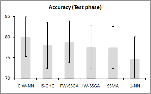
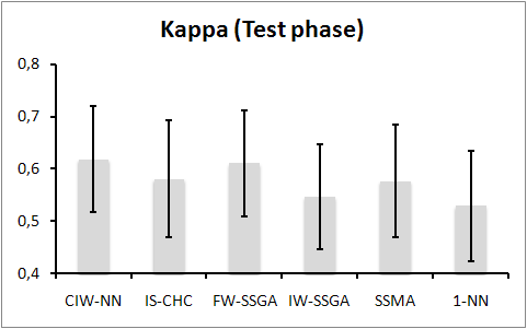
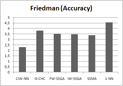
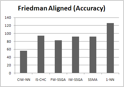
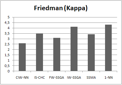
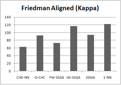
These results can also be contrasted by Friedman and Friedman Aligned procedures. Tables 7, 8, 9 and 10 show the ranks and the p-values achieved by each method with respect to accuracy and kappa measures (we also provide figures depicting the ranks achieved in both procedures):
Table 7. Results of Friedman and post-hoc methods with accuracy measure.
| Using CIW-NN as control algorithm (Rank: 2.2833) | ||||
|---|---|---|---|---|
| Method | Rank | Holm | Hochberg | Finner |
| IS-CHC | 3.81670 | 0.006008 | 0.006008 | 0.003751 |
| FW-SSGA | 3.50000 | 0.035333 | 0.022773 | 0.019552 |
| IW-SSGA | 3.46670 | 0.035333 | 0.022773 | 0.019552 |
| IS-SSMA | 3.38330 | 0.035333 | 0.022773 | 0.022773 |
| 1-NN | 4.55000 | 0.000013 | 0.000013 | 0.000013 |
| Using CIW-NN as control algorithm (Rank: 56.1833) | ||||
|---|---|---|---|---|
| Method | Rank | Holm | Hochberg | Finner |
| IS-CHC | 94.3167 | 0.024159 | 0.016404 | 0.013385 |
| FW-SSGA | 82.9 | 0.024159 | 0.016404 | 0.013385 |
| IW-SSGA | 91.8333 | 0.018363 | 0.016404 | 0.011437 |
| IS-SSMA | 91.75 | 0.047052 | 0.047052 | 0.047052 |
| 1-NN | 126.0167 | 0.000001 | 0.000001 | 0.000001 |
| Using CIW-NN as control algorithm (Rank: 2.5968) | ||||
|---|---|---|---|---|
| Method | Rank | Holm | Hochberg | Finner |
| IS-CHC | 3.4677 | 0.200462 | 0.166885 | 0.108868 |
| FW-SSGA | 3.0806 | 0.308551 | 0.308551 | 0.308551 |
| IW-SSGA | 4.1129 | 0.00568 | 0.00568 | 0.003546 |
| IS-SSMA | 3.4194 | 0.200462 | 0.166885 | 0.108868 |
| 1-NN | 4.3226 | 0.001407 | 0.001407 | 0.001406 |
| Using CIW-NN as control algorithm (Rank: 63.0806) | ||||
|---|---|---|---|---|
| Method | Rank | Holm | Hochberg | Finner |
| IS-CHC | 92.5 | 0.073941 | 0.062896 | 0.04074 |
| FW-SSGA | 73.1452 | 0.461737 | 0.461737 | 0.461737 |
| IW-SSGA | 116.4677 | 0.000378 | 0.000378 | 0.000236 |
| IS-SSMA | 93.8065 | 0.073941 | 0.062896 | 0.04074 |
| 1-NN | 122 | 0.000082 | 0.000082 | 0.000082 |
Comparison between CIW-NN and weighting methods for k-NN based classification
This subsection shows the results achieved in the experimental comparison performed between CIW-NN and weighting methods for k-NN based classification. The tables shown here can be also downloaded as an Excel document by clicking on the following link: ![]()
Tables 11 and 12 shows average accuracy results, achieved in training and test phases. Tables 13 and 14 shows average kappa results. Table 15 shows the average time elapsed and reduction rates.
Table 11. Accuracy results in training phase of the comparison between CIW-NN and weighting methods.
| CIW-NN | TS/KNN | PW | CW | CPW | ReliefF | MI | GOCBR | WDNN | ||||||||||
|---|---|---|---|---|---|---|---|---|---|---|---|---|---|---|---|---|---|---|
| Data set | Acc. | Std. | Acc. | Std. | Acc. | Std. | Acc. | Std. | Acc. | Std. | Acc. | Std. | Acc. | Std. | Acc. | Std. | Acc. | Std. |
| Australian | 85.52 | 1.05 | 89.10 | 0.84 | 84.64 | 0.35 | 81.00 | 0.88 | 83.63 | 0.95 | 83.43 | 2.36 | 82.62 | 1.72 | 89.02 | 0.53 | 89.84 | 0.49 |
| Balance | 83.64 | 1.05 | 78.95 | 0.87 | 90.10 | 0.51 | 85.05 | 0.79 | 89.85 | 1.97 | 76.84 | 0.87 | 68.84 | 4.26 | 89.21 | 0.50 | 84.89 | 0.67 |
| Bands | 71.14 | 1.82 | 80.58 | 1.61 | 82.35 | 0.79 | 79.15 | 1.39 | 82.93 | 1.67 | 72.42 | 2.56 | 57.73 | 4.63 | 82.50 | 1.24 | 73.10 | 20.33 |
| Breast | 76.30 | 1.57 | 76.93 | 1.79 | 70.39 | 1.20 | 63.85 | 2.55 | 70.71 | 1.76 | 64.10 | 4.18 | 67.75 | 2.23 | 80.77 | 0.56 | 81.20 | 1.19 |
| Bupa | 71.57 | 2.79 | 73.11 | 1.34 | 75.20 | 1.83 | 60.87 | 1.48 | 74.73 | 2.73 | 57.52 | 1.35 | 40.36 | 6.61 | 78.71 | 1.66 | 80.23 | 1.08 |
| Car | 88.58 | 2.01 | 86.09 | 0.28 | 97.66 | 0.51 | 88.00 | 1.74 | 95.10 | 0.72 | 90.83 | 0.32 | 94.91 | 0.34 | 93.63 | 0.36 | 93.82 | 0.39 |
| Cleveland | 61.64 | 1.85 | 61.86 | 3.98 | 62.01 | 1.29 | 52.26 | 0.85 | 58.00 | 1.10 | 53.39 | 1.64 | 53.54 | 1.10 | 66.45 | 0.72 | 65.38 | 1.33 |
| Contraceptive | 48.04 | 1.28 | 42.70 | 0.02 | 54.02 | 0.82 | 42.55 | 0.82 | 51.46 | 0.86 | 40.68 | 3.61 | 42.48 | 0.29 | 53.75 | 0.83 | 63.32 | 1.10 |
| Dermatology | 96.02 | 1.50 | 97.24 | 1.68 | 96.93 | 0.58 | 95.02 | 0.51 | 95.08 | 0.52 | 96.93 | 0.61 | 97.05 | 0.47 | 98.94 | 0.43 | 98.00 | 0.39 |
| German | 72.16 | 1.25 | 77.93 | 0.73 | 79.89 | 0.71 | 77.56 | 0.66 | 78.84 | 0.58 | 69.46 | 0.53 | 69.53 | 0.88 | 78.38 | 0.52 | 83.20 | 0.87 |
| Glass | 68.91 | 1.93 | 82.97 | 1.36 | 77.78 | 1.92 | 75.77 | 1.86 | 76.98 | 1.74 | 78.04 | 2.19 | 64.55 | 3.42 | 81.26 | 2.10 | 77.88 | 2.16 |
| Hayes-roth | 78.11 | 1.62 | 53.04 | 1.96 | 69.94 | 1.64 | 72.84 | 4.35 | 71.97 | 3.49 | 80.04 | 2.37 | 60.78 | 1.44 | 85.86 | 2.28 | 80.47 | 2.47 |
| Housevotes | 96.02 | 1.12 | 97.68 | 0.63 | 94.58 | 0.77 | 96.83 | 2.76 | 95.31 | 3.22 | 93.72 | 1.36 | 93.88 | 1.43 | 96.81 | 0.59 | 95.02 | 0.55 |
| Iris | 96.00 | 0.82 | 96.81 | 0.81 | 96.00 | 0.36 | 96.00 | 0.36 | 96.00 | 0.36 | 94.67 | 0.73 | 88.96 | 10.59 | 98.74 | 0.34 | 96.15 | 0.44 |
| Lymphography | 85.67 | 2.44 | 76.13 | 4.54 | 86.86 | 1.61 | 74.78 | 1.80 | 75.38 | 2.25 | 73.26 | 20.79 | 76.44 | 3.00 | 90.17 | 1.93 | 86.41 | 1.45 |
| Monk-2 | 88.45 | 2.08 | 100.00 | 0.00 | 97.93 | 1.20 | 94.49 | 1.26 | 97.82 | 4.93 | 100.00 | 0.00 | 97.22 | 0.30 | 93.75 | 0.99 | 91.64 | 0.93 |
| Movement | 61.48 | 1.37 | 74.72 | 0.54 | 84.35 | 0.63 | 86.42 | 0.63 | 85.45 | 0.63 | 13.43 | 0.61 | 75.06 | 1.07 | 87.59 | 0.41 | 89.75 | 0.58 |
| New Thyroid | 96.13 | 1.53 | 98.40 | 0.50 | 96.64 | 0.98 | 97.64 | 1.08 | 96.84 | 1.07 | 97.78 | 3.57 | 96.17 | 1.84 | 98.29 | 0.94 | 97.16 | 0.67 |
| Pima | 72.82 | 1.01 | 79.09 | 1.15 | 82.02 | 1.64 | 70.39 | 0.85 | 77.69 | 1.39 | 70.15 | 2.91 | 72.58 | 4.34 | 81.61 | 0.87 | 85.66 | 1.00 |
| Saheart | 73.38 | 1.57 | 74.72 | 1.59 | 76.98 | 1.44 | 64.50 | 1.95 | 74.46 | 1.94 | 59.72 | 4.00 | 65.08 | 2.84 | 79.08 | 0.76 | 79.53 | 0.77 |
| Sonar | 79.91 | 2.87 | 93.06 | 2.69 | 91.77 | 1.43 | 87.12 | 1.80 | 90.28 | 1.82 | 83.33 | 0.73 | 79.43 | 2.55 | 93.22 | 1.72 | 91.19 | 2.06 |
| Spectfheart | 82.98 | 2.84 | 86.06 | 4.73 | 80.40 | 2.63 | 81.58 | 2.96 | 80.74 | 2.97 | 78.19 | 3.83 | 76.45 | 0.25 | 85.48 | 2.11 | 83.90 | 2.57 |
| Tae | 55.19 | 0.91 | 38.42 | 0.57 | 62.68 | 0.84 | 58.95 | 0.21 | 59.42 | 0.21 | 45.32 | 1.36 | 34.44 | 0.82 | 73.73 | 0.43 | 72.70 | 1.08 |
| Tic-tac-toe | 75.84 | 2.06 | 73.13 | 0.76 | 85.76 | 0.84 | 84.73 | 1.07 | 84.73 | 1.16 | 87.01 | 0.82 | 85.68 | 1.13 | 86.07 | 0.95 | 80.14 | 0.56 |
| Vehicle | 66.07 | 1.12 | 77.45 | 0.17 | 80.86 | 0.25 | 79.24 | 0.22 | 79.16 | 0.26 | 72.01 | 0.18 | 70.08 | 1.27 | 77.86 | 0.31 | 82.65 | 0.24 |
| Vowel | 72.44 | 0.84 | 99.63 | 0.57 | 99.09 | 0.79 | 99.07 | 0.84 | 99.11 | 0.84 | 98.48 | 0.38 | 80.20 | 0.67 | 98.71 | 0.31 | 99.39 | 0.41 |
| Wine | 97.50 | 0.60 | 99.63 | 0.24 | 95.88 | 0.31 | 95.19 | 0.41 | 95.19 | 0.41 | 98.25 | 0.35 | 98.25 | 0.59 | 99.75 | 0.29 | 97.13 | 0.20 |
| Wisconsin | 96.71 | 1.43 | 98.00 | 0.63 | 96.71 | 0.71 | 97.93 | 0.62 | 95.14 | 0.70 | 96.79 | 1.77 | 96.37 | 2.17 | 98.52 | 0.77 | 98.03 | 0.77 |
| Yeast | 52.17 | 2.84 | 58.30 | 2.06 | 64.94 | 0.81 | 50.96 | 0.89 | 63.30 | 1.00 | 51.11 | 0.66 | 44.68 | 0.66 | 61.22 | 0.77 | 68.44 | 0.64 |
| Zoo | 90.69 | 2.04 | 66.58 | 1.52 | 93.18 | 1.99 | 92.85 | 0.96 | 93.07 | 1.50 | 95.60 | 2.87 | 95.60 | 1.50 | 97.69 | 0.93 | 96.48 | 0.83 |
| Average | 78.04 | 1.64 | 79.61 | 1.34 | 83.59 | 1.05 | 79.42 | 1.28 | 82.28 | 1.49 | 75.75 | 2.32 | 74.22 | 2.15 | 85.89 | 0.90 | 85.42 | 1.61 |
Table 12. Accuracy results in test phase of the comparison between CIW-NN and weighting methods.
| CIW-NN | TS/KNN | PW | CW | CPW | ReliefF | MI | GOCBR | WDNN | ||||||||||
|---|---|---|---|---|---|---|---|---|---|---|---|---|---|---|---|---|---|---|
| Data set | Acc. | Std. | Acc. | Std. | Acc. | Std. | Acc. | Std. | Acc. | Std. | Acc. | Std. | Acc. | Std. | Acc. | Std. | Acc. | Std. |
| Australian | 81.74 | 3.44 | 86.81 | 3.91 | 82.75 | 4.37 | 82.06 | 4.09 | 81.95 | 4.27 | 86.38 | 2.98 | 81.74 | 4.90 | 83.77 | 5.53 | 84.06 | 4.89 |
| Balance | 85.75 | 4.13 | 79.04 | 6.46 | 86.16 | 2.83 | 82.42 | 6.20 | 82.94 | 5.02 | 76.64 | 4.58 | 66.41 | 6.91 | 83.69 | 5.53 | 81.27 | 4.80 |
| Bands | 75.52 | 5.57 | 73.67 | 8.33 | 71.83 | 8.56 | 72.38 | 7.65 | 72.56 | 6.77 | 70.15 | 6.38 | 54.67 | 6.35 | 71.45 | 6.15 | 62.11 | 14.21 |
| Breast | 70.62 | 7.44 | 72.02 | 6.45 | 66.03 | 7.04 | 66.05 | 5.55 | 67.77 | 5.23 | 62.47 | 9.71 | 68.13 | 9.70 | 67.14 | 8.14 | 67.81 | 6.38 |
| Bupa | 60.95 | 7.50 | 62.44 | 7.90 | 62.13 | 9.02 | 60.79 | 7.09 | 62.37 | 6.42 | 56.46 | 4.37 | 44.27 | 8.23 | 61.81 | 6.31 | 62.82 | 6.50 |
| Car | 95.89 | 1.17 | 85.65 | 1.81 | 87.02 | 1.94 | 86.92 | 2.38 | 88.25 | 1.36 | 90.62 | 1.42 | 94.56 | 0.87 | 89.01 | 1.40 | 88.95 | 1.94 |
| Cleveland | 56.43 | 5.54 | 56.43 | 6.84 | 53.51 | 4.93 | 52.81 | 7.37 | 53.84 | 8.13 | 55.10 | 8.62 | 56.34 | 7.32 | 52.80 | 5.75 | 53.15 | 5.08 |
| Contraceptive | 45.22 | 2.59 | 42.70 | 0.22 | 44.94 | 4.72 | 42.57 | 3.56 | 44.43 | 3.29 | 39.99 | 6.05 | 42.77 | 0.90 | 43.38 | 3.65 | 44.20 | 5.14 |
| Dermatology | 96.72 | 3.17 | 96.47 | 4.01 | 95.91 | 3.28 | 95.39 | 3.09 | 95.64 | 3.09 | 95.92 | 2.77 | 96.91 | 2.32 | 96.46 | 2.98 | 97.01 | 4.10 |
| German | 72.10 | 2.51 | 71.40 | 2.20 | 71.78 | 3.41 | 72.03 | 2.69 | 72.41 | 2.70 | 69.30 | 1.42 | 68.60 | 3.41 | 70.30 | 5.37 | 71.20 | 4.26 |
| Glass | 75.72 | 11.13 | 76.42 | 13.21 | 73.65 | 12.41 | 71.98 | 11.91 | 73.31 | 11.57 | 80.65 | 12.04 | 62.44 | 6.93 | 67.67 | 14.10 | 72.66 | 13.28 |
| Hayes-roth | 72.15 | 12.73 | 54.36 | 11.56 | 67.54 | 7.72 | 71.26 | 10.55 | 69.67 | 7.68 | 80.20 | 10.67 | 60.47 | 12.69 | 67.49 | 10.55 | 70.07 | 8.85 |
| Housevotes | 94.93 | 4.12 | 95.16 | 3.34 | 94.30 | 6.33 | 93.50 | 4.95 | 94.74 | 4.98 | 94.00 | 3.48 | 94.35 | 5.49 | 92.83 | 6.27 | 91.92 | 6.14 |
| Iris | 93.33 | 5.96 | 94.00 | 4.67 | 94.00 | 5.16 | 94.00 | 5.54 | 94.67 | 5.16 | 94.00 | 5.54 | 86.67 | 8.43 | 94.00 | 3.59 | 93.33 | 6.67 |
| Lymphography | 79.30 | 12.22 | 74.54 | 8.95 | 78.63 | 9.29 | 74.52 | 10.95 | 74.52 | 10.95 | 70.43 | 22.52 | 71.90 | 10.64 | 79.34 | 9.46 | 78.55 | 10.16 |
| Monk-2 | 100.00 | 0.00 | 100.00 | 0.00 | 94.61 | 6.11 | 93.15 | 3.21 | 92.47 | 6.67 | 100.00 | 0.00 | 97.27 | 2.65 | 79.21 | 7.15 | 77.91 | 4.39 |
| Movement | 83.06 | 3.32 | 71.11 | 3.12 | 82.78 | 2.26 | 81.94 | 2.26 | 81.67 | 2.26 | 11.11 | 3.03 | 72.22 | 3.79 | 81.94 | 3.29 | 86.11 | 3.01 |
| New Thyroid | 95.82 | 3.15 | 93.48 | 2.95 | 97.23 | 4.90 | 97.23 | 3.60 | 97.23 | 3.58 | 97.25 | 4.33 | 93.03 | 3.27 | 94.87 | 4.50 | 96.75 | 3.73 |
| Pima | 71.24 | 2.03 | 75.53 | 5.85 | 71.11 | 5.96 | 69.97 | 3.87 | 72.38 | 6.68 | 70.32 | 5.65 | 67.85 | 7.01 | 70.59 | 4.88 | 73.20 | 4.39 |
| Saheart | 65.37 | 5.33 | 68.22 | 11.35 | 63.84 | 6.22 | 64.52 | 9.94 | 63.85 | 9.94 | 60.83 | 9.15 | 60.43 | 8.26 | 66.45 | 14.20 | 67.53 | 9.77 |
| Sonar | 87.00 | 3.38 | 82.10 | 6.19 | 86.85 | 4.26 | 85.41 | 7.20 | 86.52 | 7.90 | 83.57 | 3.47 | 74.52 | 9.55 | 83.55 | 8.84 | 84.55 | 8.45 |
| Spectfheart | 77.92 | 13.60 | 76.01 | 10.12 | 72.02 | 8.77 | 70.81 | 9.73 | 74.01 | 8.77 | 78.30 | 11.92 | 72.72 | 2.24 | 74.99 | 6.87 | 73.03 | 11.62 |
| Tae | 65.71 | 3.26 | 30.54 | 2.56 | 61.83 | 3.93 | 60.37 | 1.34 | 62.45 | 1.34 | 49.12 | 3.77 | 34.42 | 3.41 | 55.00 | 3.98 | 59.75 | 1.79 |
| Tic-tac-toe | 87.37 | 3.34 | 73.07 | 1.35 | 79.12 | 4.04 | 77.86 | 5.09 | 81.03 | 4.72 | 86.43 | 4.13 | 86.74 | 2.75 | 81.10 | 4.43 | 77.14 | 3.26 |
| Vehicle | 71.28 | 0.79 | 72.46 | 0.64 | 70.81 | 0.81 | 70.51 | 0.81 | 71.82 | 0.81 | 72.56 | 0.91 | 67.73 | 5.46 | 67.73 | 1.80 | 68.32 | 0.88 |
| Vowel | 98.28 | 3.78 | 98.99 | 6.79 | 99.39 | 5.25 | 99.39 | 4.97 | 99.39 | 4.97 | 98.69 | 2.65 | 77.47 | 2.80 | 96.77 | 3.36 | 99.19 | 4.85 |
| Wine | 97.16 | 2.46 | 92.09 | 2.98 | 96.78 | 2.59 | 96.32 | 3.73 | 97.03 | 3.27 | 98.27 | 3.74 | 97.71 | 3.05 | 95.49 | 2.21 | 95.52 | 1.60 |
| Wisconsin | 96.00 | 2.84 | 96.00 | 3.61 | 96.81 | 3.56 | 96.36 | 3.82 | 96.42 | 2.31 | 96.28 | 2.14 | 95.63 | 3.65 | 97.14 | 3.30 | 96.42 | 2.42 |
| Yeast | 52.76 | 3.89 | 55.86 | 12.99 | 52.29 | 6.89 | 50.67 | 5.48 | 52.16 | 5.48 | 51.55 | 4.97 | 44.34 | 4.97 | 53.44 | 6.50 | 53.50 | 4.73 |
| Zoo | 97.50 | 3.61 | 66.25 | 8.07 | 94.65 | 5.24 | 93.47 | 4.52 | 95.14 | 3.97 | 96.83 | 2.78 | 96.83 | 4.97 | 96.17 | 5.16 | 97.67 | 3.93 |
| Average | 80.09 | 4.80 | 75.76 | 5.61 | 78.34 | 5.39 | 77.56 | 5.44 | 78.42 | 5.31 | 75.78 | 5.51 | 72.97 | 5.43 | 77.19 | 5.84 | 77.52 | 5.71 |
Table 13. Kappa results in training phase of the comparison between CIW-NN and weighting methods.
| CIW-NN | TS/KNN | PW | CW | CPW | ReliefF | MI | GOCBR | WDNN | ||||||||||
|---|---|---|---|---|---|---|---|---|---|---|---|---|---|---|---|---|---|---|
| Data set | Acc. | Std. | Acc. | Std. | Acc. | Std. | Acc. | Std. | Acc. | Std. | Acc. | Std. | Acc. | Std. | Acc. | Std. | Acc. | Std. |
| Australian | .7084 | .0223 | .7799 | .0230 | .6900 | .0190 | .6150 | .0182 | .6275 | .0198 | .6646 | .0273 | .6464 | .0245 | .7778 | .0203 | .7944 | .0216 |
| Balance | .6972 | .0167 | .6308 | .0185 | .8163 | .0137 | .8076 | .0142 | .8219 | .0143 | .5934 | .0171 | .5227 | .0158 | .8007 | .0143 | .7221 | .0176 |
| Bands | .3734 | .0277 | .5983 | .0275 | .6328 | .0230 | .4403 | .0274 | .4530 | .0238 | .4230 | .0344 | .2036 | .0342 | .6376 | .0283 | .5041 | .0270 |
| Breast | .3134 | .0502 | .3515 | .0524 | .2422 | .0431 | .2210 | .0419 | .2327 | .0503 | .1405 | .0436 | .2235 | .0560 | .4916 | .0505 | .4910 | .0532 |
| Bupa | .3277 | .0355 | .4350 | .0313 | .4831 | .0341 | .4934 | .0363 | .4833 | .0347 | .0321 | .0411 | -.1277 | .0375 | .5593 | .0360 | .5874 | .0358 |
| Car | .7475 | .0085 | .6647 | .0091 | .9487 | .0071 | .9512 | .0085 | .9528 | .0085 | .7963 | .0087 | .8880 | .0079 | .8559 | .0071 | .8609 | .0082 |
| Cleveland | .3466 | .0188 | .3441 | .0175 | .3978 | .0174 | .3616 | .0192 | .3928 | .0153 | .2586 | .0157 | .2660 | .0178 | .4541 | .0220 | .4417 | .0182 |
| Contraceptive | .1598 | .0146 | .0000 | .0152 | .2869 | .0140 | .2669 | .0127 | .2713 | .0139 | .0906 | .0140 | .0053 | .0176 | .2850 | .0122 | .4306 | .0139 |
| Dermatology | .9502 | .0078 | .9654 | .0080 | .9616 | .0081 | .9578 | .0082 | .9586 | .0076 | .9616 | .0086 | .9630 | .0070 | .9867 | .0093 | .9749 | .0084 |
| German | .3943 | .0176 | .4220 | .0160 | .4984 | .0163 | .0555 | .0168 | .0589 | .0150 | .0206 | .0197 | .2651 | .0202 | .4465 | .0155 | .5655 | .0172 |
| Glass | .5564 | .0338 | .7687 | .0387 | .6978 | .0309 | .6043 | .0323 | .6804 | .0353 | .7038 | .0384 | .5058 | .0348 | .7422 | .0376 | .6972 | .0330 |
| Hayes-roth | .6657 | .0380 | .2638 | .0423 | .0180 | .0361 | .0779 | .0342 | .0179 | .0340 | .6902 | .0406 | .3954 | .0435 | .7814 | .0447 | .6980 | .0392 |
| Housevotes | .9166 | .0226 | .9511 | .0233 | .8867 | .0204 | .8770 | .0230 | .9156 | .0232 | .8676 | .0213 | .8772 | .0245 | .9328 | .0229 | .8954 | .0238 |
| Iris | .9400 | .0104 | .9522 | .0091 | .9400 | .0106 | .9400 | .0104 | .9400 | .0098 | .9300 | .0084 | .8544 | .0092 | .9811 | .0097 | .9422 | .0106 |
| Lymphography | .7165 | .0474 | .5401 | .0427 | .7448 | .0457 | .5250 | .0420 | .5359 | .0490 | .5212 | .0540 | .5523 | .0592 | .8096 | .0508 | .7360 | .0489 |
| Monk-2 | .7688 | .0248 | 1.0000 | .0000 | .8505 | .0217 | .8898 | .0238 | .8754 | .0205 | 1.0000 | .0000 | .9444 | .0305 | .8745 | .0201 | .8318 | .0259 |
| Movement | .5873 | .0165 | .7292 | .0153 | .8323 | .0158 | .8009 | .0158 | .8012 | .0157 | .0724 | .0140 | .9159 | .0171 | .8671 | .0166 | .8902 | .0158 |
| New Thyroid | .9147 | .0186 | .9655 | .0182 | .9279 | .0192 | .9279 | .0161 | .9279 | .0157 | .9528 | .0149 | .4171 | .0204 | .9631 | .0170 | .9388 | .0171 |
| Pima | .3708 | .0305 | .5233 | .0314 | .6012 | .0318 | .6345 | .0252 | .6043 | .0256 | .3055 | .0278 | .2368 | .0327 | .5852 | .0335 | .6782 | .0312 |
| Saheart | .3541 | .0203 | .3981 | .0221 | .4751 | .0192 | .4793 | .0175 | .4281 | .0170 | .0746 | .0212 | .5877 | .0192 | .5138 | .0195 | .5266 | .0213 |
| Sonar | .5973 | .0231 | .8600 | .0241 | .8341 | .0191 | .8241 | .0190 | .8375 | .0212 | .6656 | .0199 | .3014 | .0190 | .8636 | .0285 | .8223 | .0250 |
| Spectfheart | .4977 | .0733 | .4977 | .0818 | .3192 | .0648 | .3009 | .0624 | .3189 | .0710 | -.0231 | .0818 | .0000 | .0772 | .5222 | .0811 | .4356 | .0740 |
| Tae | .3277 | .0589 | .0845 | .0542 | .1392 | .0513 | .1283 | .0472 | .1502 | .0474 | .1796 | .0505 | .6769 | .0668 | .6057 | .0482 | .5899 | .0624 |
| Tic-tac-toe | .4321 | .0226 | .2746 | .0255 | .6707 | .0199 | .6907 | .0226 | .6997 | .0224 | .7092 | .0245 | .6010 | .0183 | .6655 | .0244 | .4931 | .0231 |
| Vehicle | .5478 | .0187 | .6992 | .0172 | .7448 | .0190 | .5897 | .0157 | .6417 | .0154 | .6267 | .0222 | .7022 | .0220 | .7047 | .0196 | .7686 | .0176 |
| Vowel | .6968 | .0029 | .9959 | .0032 | .9900 | .0024 | .9898 | .0027 | .9902 | .0027 | .9833 | .0029 | .9735 | .0024 | .9858 | .0025 | .9933 | .0026 |
| Wine | .9621 | .0132 | .9943 | .0147 | .9378 | .0127 | .9275 | .0112 | .9275 | .0112 | .9735 | .0115 | .9202 | .0154 | .9962 | .0144 | .9566 | .0136 |
| Wisconsin | .9274 | .0096 | .9559 | .0090 | .9273 | .0100 | .8864 | .0090 | .8912 | .0078 | .9285 | .0111 | .2919 | .0096 | .9675 | .0096 | .9567 | .0094 |
| Yeast | .3789 | .0094 | .4588 | .0086 | .5464 | .0090 | .5186 | .0089 | .5226 | .0091 | .3684 | .0117 | .9419 | .0106 | .4987 | .0076 | .5918 | .0104 |
| Zoo | .8768 | .0124 | .5092 | .0128 | .9099 | .0117 | .9056 | .0126 | .9085 | .0111 | .9419 | .0132 | .7328 | .0101 | .9695 | .0147 | .9535 | .0112 |
| Average | .6018 | .0242 | .6205 | .0238 | .6651 | .0222 | .6230 | .0218 | .6289 | .0223 | .5484 | .0240 | .5428 | .0260 | .7375 | .0246 | .7256 | .0246 |
Table 14. Kappa results in test phase of the comparison between CIW-NN and weighting methods.
| CIW-NN | TS/KNN | PW | CW | CPW | ReliefF | MI | GOCBR | WDNN | ||||||||||
|---|---|---|---|---|---|---|---|---|---|---|---|---|---|---|---|---|---|---|
| Data set | Acc. | Std. | Acc. | Std. | Acc. | Std. | Acc. | Std. | Acc. | Std. | Acc. | Std. | Acc. | Std. | Acc. | Std. | Acc. | Std. |
| Australian | .6304 | .0855 | .7338 | .1079 | .5816 | .1122 | .5606 | .1039 | .5572 | .1107 | .7251 | .1150 | .6291 | .1078 | .6726 | .1108 | .6775 | .1175 |
| Balance | .7357 | .1004 | .6351 | .1040 | .7542 | .1085 | .7108 | .1017 | .7276 | .1137 | .5897 | .1032 | .4883 | .1366 | .7038 | .1126 | .6615 | .1202 |
| Bands | .4847 | .1386 | .4547 | .1203 | .4148 | .1398 | .4435 | .1443 | .4450 | .1361 | .3737 | .1578 | .1489 | .1353 | .4093 | .1616 | .2732 | .1387 |
| Breast | .2006 | .1693 | .2203 | .1606 | .1315 | .1649 | .1249 | .1682 | .1592 | .1834 | .1024 | .1903 | .2352 | .1636 | .1367 | .1526 | .1353 | .1837 |
| Bupa | .1629 | .1475 | .2102 | .1670 | .1718 | .1767 | .1836 | .1672 | .1571 | .1591 | .0037 | .2089 | -.0426 | .1857 | .2263 | .2181 | .2300 | .1823 |
| Car | .9109 | .0458 | .6538 | .0473 | .7395 | .0441 | .7431 | .0471 | .7352 | .0414 | .7910 | .0573 | .8801 | .0486 | .7471 | .0445 | .7425 | .0418 |
| Cleveland | .2672 | .1177 | .2589 | .1148 | .2501 | .1137 | .2762 | .1223 | .2659 | .1208 | .2875 | .1180 | .3127 | .1213 | .2418 | .1078 | .2525 | .1093 |
| Contraceptive | .1202 | .0625 | .0000 | .0607 | .1275 | .0612 | .1271 | .0627 | .1254 | .0651 | .0799 | .0838 | .0089 | .0770 | .1253 | .0629 | .1371 | .0622 |
| Dermatology | .9588 | .0424 | .9557 | .0490 | .9487 | .0525 | .9350 | .0507 | .9350 | .0508 | .9489 | .0637 | .9613 | .0548 | .9556 | .0440 | .9625 | .0535 |
| German | .2712 | .0940 | .2565 | .0758 | .2694 | .0922 | .2350 | .0921 | .2399 | .0885 | .0085 | .1131 | .2416 | .1002 | .2661 | .0915 | .2509 | .0991 |
| Glass | .6640 | .1584 | .6824 | .1600 | .6099 | .1733 | .6400 | .1765 | .6239 | .1746 | .7407 | .1546 | .4745 | .1630 | .5558 | .1922 | .6273 | .1839 |
| Hayes-roth | .5587 | .1815 | .2810 | .1531 | .5031 | .1873 | .4867 | .1640 | .5186 | .1671 | .6727 | .1615 | .4109 | .1943 | .4656 | .1528 | .5115 | .1961 |
| Housevotes | .8930 | .1314 | .8979 | .1184 | .8370 | .1373 | .8680 | .1342 | .8721 | .1312 | .8747 | .1266 | .8852 | .1238 | .8499 | .1727 | .8321 | .1486 |
| Iris | .9000 | .0750 | .9166 | .0753 | .9166 | .0864 | .9166 | .0935 | .9333 | .0944 | .9166 | .0749 | .8567 | .1124 | .9166 | .0980 | .9000 | .0899 |
| Lymphography | .5944 | .1728 | .5009 | .1940 | .5788 | .1990 | .5217 | .1944 | .5217 | .2082 | .4708 | .1867 | .4593 | .2297 | .5941 | .1801 | .5817 | .1849 |
| Monk-2 | 1.0000 | .0000 | 1.0000 | .0000 | .8720 | .1228 | .8620 | .1243 | .8479 | .1248 | 1.0000 | .0000 | .9451 | .1162 | .5799 | .1605 | .5477 | .1226 |
| Movement | .8180 | .0478 | .6893 | .0523 | .8150 | .0567 | .8060 | .0514 | .8030 | .0537 | .0470 | .0555 | .8457 | .0675 | .8061 | .0642 | .8507 | .0575 |
| New Thyroid | .9112 | .0503 | .8579 | .0444 | .9410 | .0452 | .9410 | .0489 | .9410 | .0509 | .9428 | .0463 | .3120 | .0525 | .8850 | .0524 | .9281 | .0524 |
| Pima | .3329 | .0685 | .4445 | .0648 | .3473 | .0763 | .3319 | .0736 | .3184 | .0798 | .3025 | .0771 | .1164 | .0829 | .3344 | .0949 | .3944 | .0851 |
| Saheart | .1605 | .0903 | .2360 | .0807 | .1847 | .0848 | .1931 | .0947 | .2074 | .0960 | .0995 | .0784 | .4891 | .0803 | .2285 | .1160 | .2533 | .0964 |
| Sonar | .7395 | .1567 | .5657 | .1593 | .7566 | .1843 | .7259 | .1806 | .7559 | .1773 | .6698 | .2280 | .2107 | .1934 | .6663 | .1836 | .6881 | .1850 |
| Spectfheart | .2408 | .2297 | .2045 | .2077 | .1041 | .2327 | .1049 | .2444 | .1135 | .2383 | -.0193 | .2107 | .0000 | .1925 | .2074 | .1984 | .0932 | .2322 |
| Tae | .4827 | .1276 | -.0595 | .1406 | .3331 | .1438 | .3309 | .1321 | .3453 | .1292 | .1677 | .1728 | .6984 | .1583 | .1336 | .1575 | .0233 | .1447 |
| Tic-tac-toe | .7135 | .0843 | .2697 | .0828 | .6235 | .0932 | .6535 | .0870 | .6835 | .0970 | .6951 | .1129 | .5696 | .0966 | .5345 | .1147 | .4034 | .0862 |
| Vehicle | .6171 | .0721 | .6326 | .0729 | .5917 | .0777 | .5978 | .0822 | .6017 | .0839 | .6340 | .0851 | .6122 | .0662 | .5695 | .0771 | .5774 | .0872 |
| Vowel | .9811 | .0086 | .9889 | .0090 | .9933 | .0089 | .9933 | .0087 | .9933 | .0085 | .9856 | .0100 | .9651 | .0093 | .9644 | .0099 | .9911 | .0091 |
| Wine | .9567 | .0702 | .8804 | .0697 | .9244 | .0786 | .9155 | .0711 | .9155 | .0786 | .9737 | .0634 | .9039 | .0767 | .9320 | .0755 | .9327 | .0798 |
| Wisconsin | .9121 | .0594 | .9114 | .0435 | .9085 | .0532 | .8848 | .0495 | .8915 | .0509 | .9170 | .0496 | .2863 | .0453 | .9374 | .0656 | .9217 | .0592 |
| Yeast | .3885 | .0488 | .4276 | .0422 | .3816 | .0442 | .3650 | .0480 | .3770 | .0474 | .3729 | .0516 | .9597 | .0546 | .3983 | .0464 | .3982 | .0493 |
| Zoo | .9683 | .0851 | .4727 | .0820 | .9147 | .0986 | .9123 | .0909 | .9423 | .0929 | .9597 | .0813 | .7015 | .0997 | .9520 | .0943 | .9701 | .1055 |
| Average | .6192 | .0974 | .5393 | .0953 | .5842 | .1083 | .5797 | .1070 | .5851 | .1085 | .5445 | .1079 | .5189 | .1115 | .5665 | .1138 | .5583 | .1121 |
Table 15. Time elapsed and reduction rates achieved in the comparison between CIW-NN and weighting methods.
| CIW-NN | TS/KNN | PW | CW | CPW | ReliefF | MI | GOCBR | WDNN | |||
|---|---|---|---|---|---|---|---|---|---|---|---|
| Data set | Time | Reduction | Time | Time | Time | Time | Time | Time | Time | Time | Reduction |
| Australian | 63.92 | 0.9366 | 629.25 | 0.83 | 0.86 | 0.45 | 6.39 | 0.31 | 255.78 | 17.39 | 0.9594 |
| Balance | 37.34 | 0.9424 | 363.85 | 0.70 | 0.23 | 1.04 | 3.79 | 0.18 | 138.49 | 9.93 | 0.9456 |
| Bands | 64.50 | 0.9549 | 444.80 | 0.98 | 1.11 | 1.01 | 4.67 | 0.25 | 225.74 | 14.92 | 0.9357 |
| Breast | 7.36 | 0.9786 | 88.00 | 0.20 | 0.07 | 0.34 | 1.02 | 0.09 | 45.61 | 1.13 | 0.9273 |
| Bupa | 10.24 | 0.9536 | 119.64 | 0.44 | 0.05 | 0.34 | 1.34 | 0.09 | 60.29 | 2.26 | 0.9317 |
| Car | 440.59 | 0.8378 | 2672.72 | 3.26 | 3.69 | 2.84 | 28.48 | 0.19 | 1158.41 | 199.12 | 0.9503 |
| Cleveland | 9.16 | 0.9714 | 72.44 | 0.41 | 0.49 | 0.38 | 1.44 | 0.12 | 50.69 | 1.51 | 0.9487 |
| Contraceptive | 481.18 | 0.8436 | 1477.58 | 5.41 | 1.65 | 0.77 | 22.12 | 0.30 | 937.07 | 179.39 | 0.8174 |
| Dermatology | 34.60 | 0.9602 | 166.73 | 0.27 | 0.73 | 0.50 | 2.90 | 0.21 | 126.78 | 5.60 | 0.9566 |
| German | 299.23 | 0.8913 | 926.73 | 3.82 | 1.00 | 0.97 | 15.21 | 0.26 | 665.69 | 41.85 | 0.7701 |
| Glass | 5.47 | 0.9325 | 31.79 | 0.18 | 0.04 | 0.26 | 0.72 | 0.04 | 22.85 | 0.84 | 0.8724 |
| Hayes-roth | 3.59 | 0.9192 | 9.64 | 0.04 | 0.07 | 0.02 | 0.35 | 0.02 | 9.85 | 0.22 | 0.8368 |
| Housevotes | 34.05 | 0.9780 | 160.23 | 0.25 | 0.31 | 0.33 | 3.05 | 0.26 | 109.86 | 3.46 | 0.9742 |
| Iris | 3.68 | 0.9637 | 13.06 | 0.03 | 0.07 | 0.06 | 0.43 | 0.05 | 10.52 | 0.53 | 0.9400 |
| Lymphography | 3.45 | 0.9423 | 19.29 | 0.17 | 0.22 | 0.24 | 0.53 | 0.04 | 15.42 | 0.31 | 0.8919 |
| Monk-2 | 26.79 | 0.9329 | 113.74 | 0.22 | 0.59 | 0.67 | 2.00 | 0.16 | 75.82 | 5.20 | 0.8765 |
| Movement | 57.23 | 0.7469 | 572.89 | 0.55 | 2.00 | 1.27 | 8.33 | 0.11 | 279.35 | 16.18 | 0.7812 |
| New Thyroid | 6.75 | 0.9695 | 27.06 | 0.03 | 0.05 | 0.03 | 0.64 | 0.06 | 18.99 | 0.98 | 0.9483 |
| Pima | 105.56 | 0.9209 | 399.38 | 1.32 | 0.20 | 1.26 | 6.65 | 0.25 | 259.52 | 17.60 | 0.9534 |
| Saheart | 22.16 | 0.9634 | 145.44 | 0.89 | 0.10 | 0.73 | 2.58 | 0.14 | 94.53 | 4.92 | 0.9552 |
| Sonar | 18.46 | 0.9167 | 127.47 | 0.27 | 0.26 | 0.29 | 1.71 | 0.08 | 65.68 | 1.17 | 0.8964 |
| Spectfheart | 17.89 | 0.9817 | 182.47 | 0.45 | 0.17 | 0.21 | 2.06 | 0.11 | 79.82 | 0.87 | 0.9795 |
| Tae | 3.93 | 0.9382 | 21.18 | 0.03 | 0.03 | 0.04 | 0.44 | 0.04 | 12.36 | 0.33 | 0.7513 |
| Tic-tac-toe | 134.31 | 0.8867 | 979.65 | 2.46 | 0.51 | 0.50 | 10.35 | 0.30 | 378.87 | 34.16 | 0.9328 |
| Vehicle | 123.21 | 0.9028 | 1040.90 | 2.48 | 0.61 | 1.05 | 10.35 | 0.19 | 431.97 | 49.56 | 0.8882 |
| Vowel | 303.91 | 0.7497 | 1221.17 | 0.23 | 0.38 | 0.41 | 11.78 | 0.29 | 532.80 | 143.09 | 0.7277 |
| Wine | 5.61 | 0.9688 | 39.70 | 0.05 | 0.21 | 0.05 | 0.60 | 0.04 | 17.79 | 0.71 | 0.7631 |
| Wisconsin | 86.64 | 0.9474 | 525.34 | 0.40 | 0.94 | 1.06 | 5.73 | 0.31 | 213.67 | 16.15 | 0.9871 |
| Yeast | 487.48 | 0.8349 | 2485.15 | 6.77 | 0.32 | 9.68 | 26.03 | 0.21 | 953.38 | 184.99 | 0.9415 |
| Zoo | 3.80 | 0.8999 | 14.90 | 0.02 | 0.03 | 0.04 | 0.52 | 0.03 | 8.58 | 0.22 | 0.8461 |
| Average | 96.74 | 0.9189 | 503.07 | 1.11 | 0.57 | 0.89 | 6.07 | 0.16 | 241.87 | 31.82 | 0.8962 |
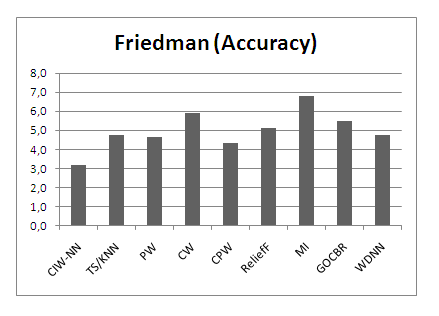
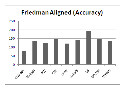
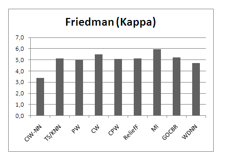
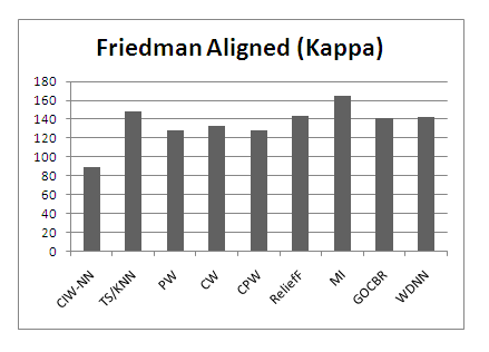
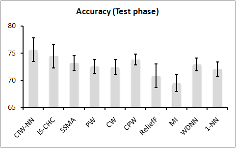
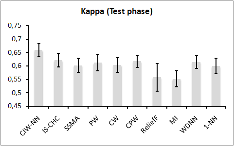
The results achieved in test phase can be viewed graphycally. The following pictures depict the average accuracy and kappa results (with standard deviations) achieved by each configuration:
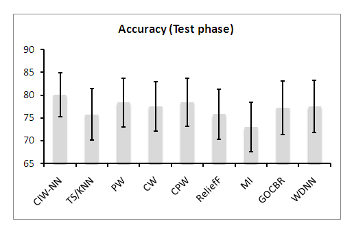
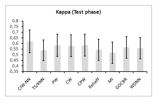
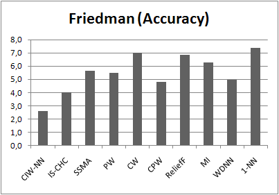
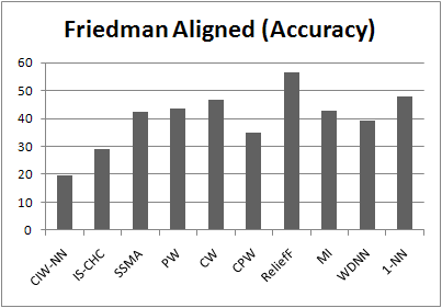
These results can also be contrasted by Friedman and Friedman Aligned procedures. Tables 16, 17, 18 and 19 show the ranks and the p-values achieved by each method with respect to accuracy and kappa measures (we also provide figures depicting the ranks achieved in both procedures):
| Using CIW-NN as control algorithm (Rank: 3.167) | ||||
|---|---|---|---|---|
| Method | Rank | Holm | Hochberg | Finner |
| TS/KNN | 4.767 | 0.09461 | 0.07095 | 0.03757 |
| PW | 4.633 | 0.09461 | 0.07613 | 0.04338 |
| CW | 5.933 | 0.00064 | 0.00064 | 0.00037 |
| CPW | 4.333 | 0.09896 | 0.09896 | 0.09896 |
| ReliefF | 5.117 | 0.02910 | 0.02910 | 0.01161 |
| MI | 6.783 | 0.00000 | 0.00000 | 0.00000 |
| GOCBR | 5.500 | 0.00580 | 0.00580 | 0.00258 |
| WDNN | 4.767 | 0.09461 | 0.07095 | 0.03757 |
| Using CIW-NN as control algorithm (Rank: 79.733) | ||||
|---|---|---|---|---|
| Method | Rank | Holm | Hochberg | Finner |
| TS/KNN | 136.700 | 0.01888 | 0.01800 | 0.00754 |
| PW | 125.050 | 0.04920 | 0.04500 | 0.02806 |
| CW | 147.333 | 0.00560 | 0.00560 | 0.00320 |
| CPW | 120.150 | 0.04920 | 0.04500 | 0.04500 |
| ReliefF | 140.350 | 0.01321 | 0.01321 | 0.00528 |
| MI | 190.483 | 0.00000 | 0.00000 | 0.00000 |
| GOCBR | 144.567 | 0.00781 | 0.00781 | 0.00347 |
| WDNN | 135.133 | 0.01888 | 0.01800 | 0.00799 |
| Using CIW-NN as control algorithm (Rank: 3.383) | ||||
|---|---|---|---|---|
| Method | Rank | Holm | Hochberg | Finner |
| TS/KNN | 5.100 | 0.07597 | 0.04863 | 0.03016 |
| PW | 4.967 | 0.07597 | 0.05029 | 0.03016 |
| CW | 5.483 | 0.02086 | 0.02086 | 0.01186 |
| CPW | 5.083 | 0.07597 | 0.04863 | 0.03016 |
| ReliefF | 5.100 | 0.07597 | 0.04863 | 0.03016 |
| MI | 5.933 | 0.00249 | 0.00249 | 0.00248 |
| GOCBR | 5.233 | 0.05333 | 0.04863 | 0.02353 |
| WDNN | 4.717 | 0.07597 | 0.05935 | 0.05935 |
| Using CIW-NN as control algorithm (Rank: 88.750) | ||||
|---|---|---|---|---|
| Method | Rank | Holm | Hochberg | Finner |
| TS/KNN | 147.867 | 0.02357 | 0.02357 | 0.01340 |
| PW | 128.033 | 0.10019 | 0.05137 | 0.05704 |
| CW | 133.417 | 0.08020 | 0.05137 | 0.03548 |
| CPW | 128.250 | 0.10019 | 0.05137 | 0.05704 |
| ReliefF | 143.933 | 0.03720 | 0.03572 | 0.01645 |
| MI | 165.300 | 0.00117 | 0.00117 | 0.00117 |
| GOCBR | 141.467 | 0.03848 | 0.03572 | 0.01645 |
| WDNN | 142.483 | 0.03848 | 0.03572 | 0.01645 |
Study of the behavior of CIW-NN in large-sized domains
This subsection shows the results achieved in the experimental comparison performed in large domains. The tables shown here can be also downloaded as an Excel document by clicking on the following link: ![]()
Tables 20 and 21 shows average accuracy results, achieved in training and test phases. Tables 22 and 23 shows average kappa results. Table 24 shows the average time elapsed and reduction rates.
Table 20. Accuracy results in training phase of the comparison performed in large domains.
| CIW-NN | IS-CHC | SSMA | PW | CW | CPW | ReliefF | MI | WDNN | 1-NN | |||||||||||
|---|---|---|---|---|---|---|---|---|---|---|---|---|---|---|---|---|---|---|---|---|
| Data set | Acc. | Std. | Acc. | Std. | Acc. | Std. | Acc. | Std. | Acc. | Std. | Acc. | Std. | Acc. | Std. | Acc. | Std. | Acc. | Std. | Acc. | Std. |
| Abalone | 24.09 | 0.57 | 24.09 | 0.57 | 34.44 | 0.63 | 33.04 | 0.78 | 19.91 | 0.32 | 33.16 | 0.68 | 14.85 | 0.83 | 3.16 | 2.06 | 36.29 | 0.81 | 19.87 | 0.31 |
| Banana | 88.15 | 0.26 | 88.15 | 0.26 | 91.50 | 0.22 | 87.27 | 0.18 | 87.11 | 0.19 | 87.27 | 0.18 | 69.42 | 2.45 | 87.08 | 0.24 | 93.05 | 0.12 | 87.11 | 0.20 |
| Chess | 96.56 | 1.45 | 96.56 | 1.45 | 93.39 | 0.80 | 94.38 | 0.27 | 47.84 | 0.06 | 47.84 | 0.06 | 95.77 | 0.19 | 96.08 | 1.19 | 94.35 | 0.28 | 84.45 | 0.26 |
| Marketing | 30.70 | 0.17 | 30.68 | 0.39 | 37.13 | 0.55 | 34.93 | 0.95 | 25.96 | 0.38 | 26.20 | 0.42 | 26.97 | 0.32 | 23.33 | 2.89 | 39.78 | 0.32 | 27.50 | 0.23 |
| Page-blocks | 95.75 | 0.44 | 95.75 | 0.44 | 95.98 | 0.17 | 95.71 | 0.17 | 95.43 | 0.17 | 95.49 | 0.17 | 96.73 | 0.16 | 95.74 | 0.11 | 97.33 | 0.07 | 95.65 | 0.15 |
| Phoneme | 85.56 | 0.42 | 85.40 | 0.48 | 89.34 | 0.51 | 90.21 | 0.22 | 90.00 | 0.22 | 90.21 | 0.21 | 80.22 | 0.72 | 72.71 | 6.18 | 94.20 | 0.22 | 89.98 | 0.21 |
| Segment | 92.63 | 0.32 | 92.63 | 0.45 | 96.54 | 0.52 | 96.84 | 0.20 | 96.72 | 0.22 | 96.87 | 0.20 | 96.06 | 0.46 | 98.10 | 0.22 | 98.01 | 0.20 | 96.73 | 0.21 |
| Splice | 83.09 | 0.68 | 82.42 | 0.96 | 83.30 | 0.39 | 63.00 | 1.86 | 31.41 | 4.03 | 29.81 | 0.75 | 78.49 | 0.30 | 90.90 | 0.37 | 88.71 | 1.28 | 75.25 | 0.30 |
| Average | 74.56 | 0.54 | 74.46 | 0.63 | 77.70 | 0.47 | 74.42 | 0.58 | 61.80 | 0.70 | 63.36 | 0.33 | 69.81 | 0.68 | 70.89 | 1.66 | 80.22 | 0.41 | 72.07 | 0.24 |
Table 21. Accuracy results in test phase of the comparison performed in large domains.
| CIW-NN | IS-CHC | SSMA | PW | CW | CPW | ReliefF | MI | WDNN | 1-NN | |||||||||||
|---|---|---|---|---|---|---|---|---|---|---|---|---|---|---|---|---|---|---|---|---|
| Data set | Acc. | Std. | Acc. | Std. | Acc. | Std. | Acc. | Std. | Acc. | Std. | Acc. | Std. | Acc. | Std. | Acc. | Std. | Acc. | Std. | Acc. | Std. |
| Abalone | 22.23 | 1.33 | 25.34 | 1.33 | 26.09 | 1.41 | 22.21 | 1.41 | 20.05 | 1.51 | 22.16 | 1.49 | 14.71 | 1.85 | 3.14 | 2.07 | 20.84 | 1.75 | 19.91 | 1.52 |
| Banana | 87.62 | 1.04 | 89.42 | 1.04 | 89.64 | 0.89 | 87.61 | 0.92 | 87.49 | 0.92 | 87.54 | 0.92 | 68.53 | 2.76 | 87.45 | 0.95 | 88.74 | 0.82 | 87.51 | 0.98 |
| Chess | 98.06 | 1.05 | 86.06 | 1.05 | 90.05 | 1.67 | 86.23 | 1.57 | 87.87 | 0.21 | 89.87 | 0.21 | 96.09 | 0.57 | 96.18 | 1.66 | 85.95 | 1.47 | 84.70 | 2.24 |
| Marketing | 30.05 | 0.89 | 29.75 | 0.97 | 30.87 | 1.63 | 26.74 | 1.33 | 27.80 | 1.50 | 28.14 | 1.64 | 26.45 | 1.91 | 23.21 | 3.32 | 28.54 | 1.28 | 27.38 | 1.27 |
| Page-blocks | 96.35 | 0.82 | 95.98 | 0.82 | 95.10 | 0.83 | 95.82 | 0.90 | 95.79 | 0.94 | 96.03 | 0.89 | 96.49 | 0.41 | 95.80 | 0.82 | 96.29 | 0.50 | 95.76 | 0.96 |
| Phoneme | 91.19 | 1.47 | 90.45 | 1.53 | 85.70 | 1.33 | 89.97 | 1.59 | 89.93 | 1.66 | 89.86 | 1.66 | 79.66 | 2.39 | 72.43 | 5.36 | 89.86 | 1.34 | 89.91 | 1.66 |
| Segment | 96.28 | 9.55 | 96.18 | 9.25 | 95.11 | 1.46 | 96.63 | 0.67 | 96.09 | 0.67 | 96.67 | 0.67 | 95.71 | 1.26 | 98.23 | 0.98 | 96.97 | 0.82 | 96.62 | 0.67 |
| Splice | 83.57 | 1.37 | 82.98 | 1.37 | 73.32 | 1.63 | 75.57 | 1.87 | 74.54 | 3.75 | 80.37 | 0.69 | 78.24 | 1.30 | 90.44 | 1.97 | 76.58 | 1.48 | 74.95 | 1.09 |
| Average | 75.67 | 2.19 | 74.52 | 2.17 | 73.24 | 1.36 | 72.60 | 1.28 | 72.45 | 1.39 | 73.83 | 1.02 | 69.49 | 1.56 | 70.86 | 2.14 | 72.97 | 1.18 | 72.09 | 1.30 |
Table 22. Kappa results in training phase of the comparison performed in large domains.
| CIW-NN | IS-CHC | SSMA | PW | CW | CPW | ReliefF | MI | WDNN | 1-NN | |||||||||||
|---|---|---|---|---|---|---|---|---|---|---|---|---|---|---|---|---|---|---|---|---|
| Data set | Acc. | Std. | Acc. | Std. | Acc. | Std. | Acc. | Std. | Acc. | Std. | Acc. | Std. | Acc. | Std. | Acc. | Std. | Acc. | Std. | Acc. | Std. |
| Abalone | .1281 | .0102 | .1281 | .0103 | .2518 | .0071 | .2444 | .0092 | .1045 | .0038 | .2472 | .0082 | .0000 | .0000 | .0844 | .0045 | .2851 | .0093 | .1040 | .0037 |
| Banana | .7595 | .0053 | .7595 | .0050 | .8276 | .0044 | .7428 | .0040 | .7395 | .0041 | .7438 | .0040 | .7388 | .0051 | .4456 | .0064 | .8591 | .0026 | .7395 | .0043 |
| Chess | .9311 | .0308 | .9311 | .0337 | .8675 | .0160 | .8873 | .0058 | .8535 | .0011 | .8945 | .0011 | .9215 | .0250 | .9235 | .0059 | .8864 | .0060 | .6849 | .0055 |
| Marketing | .1832 | .0047 | .1806 | .0063 | .2702 | .0075 | .2563 | .0113 | .1613 | .0042 | .2360 | .0045 | .1272 | .0332 | .1429 | .0031 | .3119 | .0039 | .1731 | .0029 |
| Page-blocks | .7616 | .0280 | .7616 | .0290 | .7673 | .0119 | .7955 | .0109 | .7738 | .0112 | .7979 | .0113 | .7654 | .0058 | .8562 | .0099 | .8513 | .0041 | .7637 | .0085 |
| Phoneme | .6559 | .0091 | .7480 | .0116 | .7393 | .0127 | .7595 | .0058 | .7543 | .0058 | .7595 | .0054 | .0786 | .2485 | .6549 | .0071 | .8581 | .0051 | .7538 | .0056 |
| Segment | .9140 | .0104 | .9540 | .0132 | .9596 | .0060 | .9632 | .0025 | .9618 | .0027 | .9635 | .0025 | .9778 | .0027 | .9650 | .0035 | .9768 | .0017 | .9619 | .0026 |
| Splice | .7224 | .0124 | .7109 | .0169 | .7290 | .0064 | .6788 | .0475 | .6266 | .0560 | .7355 | .0104 | .8556 | .0059 | .6759 | .0064 | .8182 | .0209 | .6092 | .0049 |
| Average | .6320 | .0139 | .6467 | .0158 | .6765 | .0090 | .6660 | .0121 | .6219 | .0111 | .6722 | .0059 | .5581 | .0408 | .5936 | .0059 | .7308 | .0067 | .5988 | .0048 |
Table 23. Kappa results in test phase of the comparison performed in large domains.
| CIW-NN | IS-CHC | SSMA | PW | CW | CPW | ReliefF | MI | WDNN | 1-NN | |||||||||||
|---|---|---|---|---|---|---|---|---|---|---|---|---|---|---|---|---|---|---|---|---|
| Data set | Acc. | Std. | Acc. | Std. | Acc. | Std. | Acc. | Std. | Acc. | Std. | Acc. | Std. | Acc. | Std. | Acc. | Std. | Acc. | Std. | Acc. | Std. |
| Abalone | .1067 | .0157 | .1057 | .0178 | .1565 | .0171 | .1223 | .0173 | .1054 | .0172 | .1235 | .0185 | .0000 | .0000 | .0480 | .0200 | .1124 | .0198 | .1038 | .0174 |
| Banana | .7489 | .0224 | .7592 | .0235 | .7900 | .0181 | .7486 | .0196 | .7478 | .0197 | .7488 | .0196 | .7463 | .0202 | .3272 | .0213 | .7720 | .0174 | .7476 | .0208 |
| Chess | .9611 | .0222 | .6911 | .0231 | .8005 | .0335 | .7240 | .0334 | .7146 | .0039 | .7392 | .0039 | .9235 | .0351 | .9185 | .0456 | .7166 | .0313 | .6899 | .0484 |
| Marketing | .1792 | .0121 | .1732 | .0104 | .1974 | .0189 | .1834 | .0156 | .1596 | .0176 | .1719 | .0191 | .1260 | .0378 | .1311 | .0186 | .1841 | .0153 | .1720 | .0152 |
| Page-blocks | .8006 | .0453 | .7958 | .0484 | .7131 | .0515 | .7769 | .0551 | .7702 | .0609 | .7897 | .0578 | .7670 | .0474 | .8219 | .0648 | .7935 | .0330 | .7673 | .0584 |
| Phoneme | .7886 | .0367 | .7685 | .0385 | .6482 | .0316 | .7533 | .0435 | .7518 | .0453 | .7547 | .0455 | .0720 | .2275 | .5781 | .0491 | .7527 | .0351 | .7518 | .0453 |
| Segment | .9566 | .0129 | .9536 | .0135 | .9429 | .0171 | .9611 | .0082 | .9607 | .0082 | .9632 | .0083 | .9793 | .0120 | .9495 | .0086 | .9646 | .0112 | .9606 | .0082 |
| Splice | .7316 | .0239 | .7207 | .0241 | .5715 | .0275 | .6292 | .0482 | .6184 | .0515 | .6478 | .0094 | .8483 | .0323 | .6401 | .0154 | .6235 | .0251 | .6055 | .0185 |
| Average | .6591 | .0239 | .6210 | .0249 | .6025 | .0269 | .6124 | .0301 | .6036 | .0280 | .6173 | .0227 | .5578 | .0515 | .5518 | .0304 | .6149 | .0235 | .5998 | .0290 |
Table 24. Time elapsed and reduction rates achieved in the comparison between CIW-NN and weighting methods.
| CIW-NN | IS-CHC | SSMA | PW | CW | CPW | ReliefF | MI | WDNN | |||||
|---|---|---|---|---|---|---|---|---|---|---|---|---|---|
| Data set | Time | Reduction | Time | Reduction | Time | Reduction | Time | Time | Time | Time | Time | Time | Reduction |
| Abalone | 2190.86 | 0.8498 | 1372.49 | 0.9963 | 1282.19 | 0.9727 | 2.33 | 2.33 | 2.33 | 70.60 | 1.53 | 539.04 | 0.8755 |
| Banana | 2767.95 | 0.8499 | 1476.35 | 0.9933 | 1435.12 | 0.9879 | 3.01 | 2.93 | 3.27 | 77.85 | 1.94 | 582.74 | 0.8317 |
| Chess | 2291.09 | 0.8497 | 970.38 | 0.9936 | 887.73 | 0.9753 | 14.01 | 13.39 | 11.56 | 100.94 | 3.45 | 366.65 | 0.8667 |
| Marketing | 17050.66 | 0.8499 | 4735.82 | 0.9979 | 4672.53 | 0.9825 | 61.32 | 61.52 | 64.07 | 675.56 | 22.04 | 1622.36 | 0.8346 |
| Page-blocks | 7845.33 | 0.8498 | 1720.74 | 0.9943 | 1592.95 | 0.9916 | 12.88 | 12.92 | 13.65 | 133.03 | 5.54 | 627.06 | 0.8272 |
| Phoneme | 6746.37 | 0.8499 | 2662.28 | 0.9949 | 2635.07 | 0.9752 | 6.35 | 6.21 | 6.36 | 76.94 | 3.75 | 985.56 | 0.8281 |
| Segment | 1818.27 | 0.9284 | 547.81 | 0.9855 | 533.49 | 0.9713 | 1.12 | 0.98 | 1.36 | 23.17 | 0.91 | 229.49 | 0.8741 |
| Splice | 8372.87 | 0.8499 | 1920.97 | 0.9916 | 1883.88 | 0.9679 | 27.58 | 27.21 | 29.58 | 142.30 | 5.38 | 719.04 | 0.8530 |
| Average | 6135.42 | 0.8597 | 1925.85 | 0.9934 | 1865.37 | 0.97805 | 16.08 | 15.94 | 16.52 | 162.55 | 5.57 | 672.92 | 0.8489 |
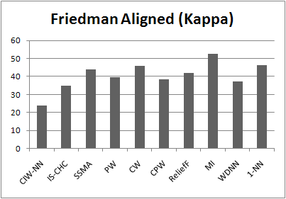
The results achieved in test phase can be viewed graphycally. The following pictures depict the average accuracy and kappa results (with standard deviations) achieved by each configuration:
These results can also be contrasted by Friedman and Friedman Aligned procedures. Tables 25, 26, 27 and 28 show the ranks and the p-values achieved by each method with respect to accuracy and kappa measures (we also provide figures depicting the ranks achieved in both procedures):
| Using CIW-NN as control algorithm (Rank: 2.630) | ||||
|---|---|---|---|---|
| Method | Rank | Holm | Hochberg | Finner |
| IS-CHC | 4.0000 | 0.3798 | 0.3637 | 0.363722 |
| SSMA | 5.6250 | 0.2375 | 0.2302 | 0.0839 |
| PW | 5.5000 | 0.2375 | 0.2302 | 0.085061 |
| CW | 7.0000 | 0.0308 | 0.0308 | 0.0172 |
| CPW | 4.8125 | 0.3798 | 0.2969 | 0.165389 |
| ReliefF | 6.8750 | 0.0350 | 0.0350 | 0.0172 |
| MI | 6.2500 | 0.0998 | 0.0998 | 0.0370 |
| WDNN | 4.9375 | 0.3798 | 0.2969 | 0.159752 |
| 1-NN | 7.3750 | 0.0153 | 0.0153 | 0.0152 |
| Using CIW-NN as control algorithm (Rank: 19.630) | ||||
|---|---|---|---|---|
| Method | Rank | Holm | Hochberg | Finner |
| IS-CHC | 28.8750 | 0.546865 | 0.546865 | 0.546865 |
| SSMA | 42.2500 | 0.367288 | 0.317996 | 0.132491 |
| PW | 43.6250 | 0.367288 | 0.317996 | 0.132491 |
| CW | 46.7500 | 0.225975 | 0.225975 | 0.105806 |
| CPW | 34.9375 | 0.521822 | 0.521822 | 0.288321 |
| ReliefF | 56.5000 | 0.025938 | 0.025938 | 0.025641 |
| MI | 42.7500 | 0.367288 | 0.317996 | 0.132491 |
| WDNN | 39.4375 | 0.391953 | 0.391953 | 0.164741 |
| 1-NN | 48.0000 | 0.196364 | 0.196364 | 0.105806 |
| Using CIW-NN as control algorithm (Rank: 3.250) | ||||
|---|---|---|---|---|
| Method | Rank | Holm | Hochberg | Finner |
| IS-CHC | 4.875 | 1.132296 | 0.56326 | 0.392968 |
| SSMA | 5.625 | 0.583387 | 0.56326 | 0.200139 |
| PW | 4.75 | 1.132296 | 0.56326 | 0.392968 |
| CW | 7.0625 | 0.094297 | 0.094297 | 0.051959 |
| CPW | 4.25 | 1.132296 | 0.56326 | 0.550652 |
| ReliefF | 6.5 | 0.190817 | 0.190817 | 0.070138 |
| MI | 6.875 | 0.116471 | 0.116471 | 0.051959 |
| WDNN | 4.125 | 1.132296 | 0.56326 | 0.56326 |
| 1-NN | 7.6875 | 0.030378 | 0.030378 | 0.029971 |
| Using CIW-NN as control algorithm (Rank: 23.875) | ||||
|---|---|---|---|---|
| Method | Rank | Holm | Hochberg | Finner |
| IS-CHC | 34.75 | 0.687376 | 0.349288 | 0.349288 |
| SSMA | 43.875 | 0.51115 | 0.349288 | 0.214181 |
| PW | 39.75 | 0.687376 | 0.349288 | 0.246353 |
| CW | 45.8125 | 0.417222 | 0.349288 | 0.214181 |
| CPW | 38.375 | 0.687376 | 0.349288 | 0.263911 |
| ReliefF | 42.125 | 0.58125 | 0.349288 | 0.214181 |
| MI | 52.75 | 0.116542 | 0.116542 | 0.110685 |
| WDNN | 37.25 | 0.687376 | 0.349288 | 0.276139 |
| 1-NN | 46.4375 | 0.417222 | 0.349288 | 0.214181 |

Additional studies
In this section, we report the results obtained in several additional studies performed with the aim of fully characterize the behaviour of CIW-NN, regarding its most sensitive charasteristics, as well as to justify several decisions taken during its development.
An excel file, summarizing all the results achieved in the additional studies, can be downloaded in the following link: ![]()
Setting up the crossover operator with multiple descendants
The definition of the crossover operator used by FW and IW populations is a critical task in the development of CIW-NN. This study is devoted to analyze several suitable combinations of operators considered, and to justify the final decision taken.
Following (A. M. Sánchez, M. Lozano, P. Villar, and F. Herrera, “Hybrid crossover operators with multiple descendents for real-coded genetic algorithms: Combining neighborhood-based crossover operators,” International Journal on Intelligent Systems, vol. 24, no. 5, pp. 540–567,2009.) as the starting point of the study, we can highlight three basic options:
- To employ a combination of different crossover operators (heterogeneous).
- To employ only one crossover operator, by combining several versions of it (homogeneous).
- To employ just one crossover operator, without multiple descendants (simple).
The concrete option selected will have a strong effect on the behavior of the SSGA algorithm, not only in the results obtained, but also in the cost of each generation (each application of the crossover operator will spend more than the two evaluations used by the classical BLX-α operator).
We have considered the two best performing configurations given in (A. M. Sánchez et al.) for each category of multiple descendants, and the basic BLX-0.5 as the baseline option. The characteristics of the configurations tested in this study are shown in Table 29:
Table 29. Configurations tested for the crossover operator with multiple descendants of CIW-NN.
| Code | Configuration | Type | #Operators | #Descendants |
|---|---|---|---|---|
| A | 2BLX0.5-2FR0.5-2PNX3-2SBX0.01 | Heterogeneous | 4 | 8 |
| B | 2BLX0.5-2PNX3-2SBX0.01 | Heterogeneous | 3 | 6 |
| C | 2BLX0.3-4BLX0.5-2BLX0.7 | Homogeneous | 4 | 8 |
| D | 2BLX0.3-2BLX0.5-2BLX0.7 | Homogeneous | 3 | 6 |
| E | 2BLX0.5 | Simple | 1 | 2 |
We have carried out an experiment on the 30 small data sets of the general framework. Due to this issue only affecting the dynamics of the IW and FW populations, we will only take into consideration in this comparison the accuracy obtained, since it is the measure which composes their fitness functions.
The results obtained can be downloaded as an Excel document by clicking on the following link: ![]()
Tables 30 and 31 shows the average accuracy results achieved in training and test phase, respectively:
| Configuration | A | B | C | D | E | |||||
|---|---|---|---|---|---|---|---|---|---|---|
| Dataset | Accuracy | Std. Dev | Accuracy | Std. Dev | Accuracy | Std. Dev | Accuracy | Std. Dev | Accuracy | Std. Dev |
| Australian | 85.75 | 1.10 | 85.46 | 1.27 | 85.52 | 1.05 | 85.62 | 0.89 | 85.81 | 1.21 |
| Balance | 84.20 | 1.10 | 82.84 | 1.40 | 83.64 | 1.05 | 83.96 | 1.45 | 84.48 | 1.03 |
| Bands | 70.65 | 1.42 | 70.40 | 1.35 | 71.14 | 1.82 | 70.13 | 1.29 | 71.28 | 0.61 |
| Breast | 74.86 | 1.27 | 75.49 | 1.69 | 76.30 | 1.57 | 76.22 | 1.81 | 76.11 | 1.72 |
| Bupa | 69.53 | 2.66 | 68.73 | 1.74 | 71.57 | 2.79 | 69.92 | 2.44 | 67.76 | 1.89 |
| Car | 89.31 | 1.15 | 89.42 | 1.10 | 88.58 | 2.01 | 89.91 | 1.85 | 89.18 | 0.81 |
| Cleveland | 61.53 | 1.70 | 62.04 | 1.34 | 61.64 | 1.85 | 61.02 | 1.54 | 60.80 | 1.79 |
| Contraceptive | 47.36 | 1.57 | 47.48 | 1.22 | 48.04 | 1.28 | 47.85 | 1.60 | 48.53 | 1.46 |
| Dermatology | 96.96 | 1.09 | 96.21 | 0.73 | 96.02 | 1.50 | 96.39 | 0.90 | 95.96 | 1.40 |
| German | 71.69 | 1.20 | 71.72 | 0.64 | 72.16 | 1.25 | 71.68 | 1.11 | 72.09 | 0.77 |
| Glass | 70.56 | 2.10 | 68.95 | 3.53 | 68.91 | 1.93 | 69.90 | 2.40 | 68.03 | 2.71 |
| Hayes-roth | 76.32 | 6.91 | 78.87 | 1.74 | 78.11 | 1.62 | 78.79 | 3.88 | 77.43 | 2.34 |
| Housevotes | 95.68 | 0.67 | 95.43 | 0.94 | 96.02 | 1.12 | 95.53 | 0.75 | 96.04 | 0.76 |
| Iris | 96.44 | 0.73 | 97.11 | 1.12 | 96.00 | 0.82 | 97.41 | 1.62 | 95.56 | 1.16 |
| Lymphography | 85.07 | 2.44 | 84.39 | 1.38 | 85.67 | 2.44 | 84.99 | 2.37 | 85.74 | 2.08 |
| Monk-2 | 86.84 | 2.12 | 89.20 | 4.07 | 88.45 | 2.08 | 86.42 | 4.97 | 87.50 | 2.29 |
| Movement | 95.71 | 1.61 | 96.18 | 1.46 | 96.13 | 1.37 | 96.33 | 1.62 | 96.64 | 1.59 |
| New Thyroid | 73.06 | 1.57 | 73.32 | 1.88 | 72.82 | 1.53 | 73.50 | 1.24 | 72.29 | 2.05 |
| Pima | 74.03 | 1.08 | 73.31 | 1.33 | 73.38 | 1.01 | 73.30 | 1.13 | 73.81 | 1.17 |
| Saheart | 79.70 | 2.13 | 78.85 | 3.02 | 79.91 | 1.57 | 78.53 | 2.69 | 78.85 | 2.85 |
| Sonar | 83.86 | 1.83 | 82.73 | 2.40 | 82.98 | 2.87 | 83.85 | 2.78 | 83.07 | 2.40 |
| Spectfheart | 55.12 | 2.37 | 57.10 | 2.89 | 55.19 | 2.84 | 55.26 | 1.68 | 55.85 | 2.71 |
| Tae | 75.11 | 1.63 | 75.01 | 1.40 | 75.84 | 0.91 | 75.71 | 1.76 | 75.53 | 2.47 |
| Tic-tac-toe | 65.33 | 0.92 | 66.39 | 1.91 | 66.07 | 2.06 | 66.05 | 1.56 | 66.26 | 2.24 |
| Vehicle | 69.73 | 0.78 | 69.73 | 0.78 | 72.44 | 1.12 | 69.73 | 0.78 | 69.73 | 0.78 |
| Vowel | 97.56 | 1.20 | 98.19 | 0.86 | 97.50 | 0.84 | 97.69 | 1.03 | 97.44 | 1.12 |
| Wine | 96.55 | 0.69 | 96.77 | 0.35 | 96.71 | 0.60 | 96.61 | 0.39 | 96.76 | 0.65 |
| Wisconsin | 51.69 | 2.02 | 51.89 | 2.05 | 52.17 | 1.43 | 52.16 | 2.02 | 53.06 | 1.10 |
| Yeast | 88.05 | 3.33 | 90.76 | 2.94 | 90.69 | 2.84 | 90.24 | 3.85 | 89.92 | 2.68 |
| Zoo | 62.56 | 3.02 | 62.31 | 2.44 | 61.48 | 2.04 | 62.84 | 2.51 | 62.35 | 2.20 |
| Average | 77.69 | 1.78 | 77.88 | 1.70 | 78.04 | 1.64 | 77.92 | 1.86 | 77.80 | 1.67 |
| Configuration | A | B | C | D | E | |||||
|---|---|---|---|---|---|---|---|---|---|---|
| Dataset | Accuracy | Std. Dev | Accuracy | Std. Dev | Accuracy | Std. Dev | Accuracy | Std. Dev | Accuracy | Std. Dev |
| Australian | 81.45 | 4.84 | 81.01 | 4.17 | 81.74 | 3.44 | 81.16 | 5.23 | 79.86 | 2.86 |
| Balance | 85.76 | 2.52 | 84.49 | 3.78 | 85.75 | 4.13 | 85.45 | 3.90 | 83.67 | 3.72 |
| Bands | 74.22 | 6.51 | 74.78 | 6.70 | 75.52 | 5.57 | 74.97 | 6.55 | 74.22 | 5.96 |
| Breast | 72.02 | 5.41 | 70.70 | 5.77 | 70.62 | 7.44 | 69.33 | 10.06 | 71.32 | 5.40 |
| Bupa | 60.56 | 9.35 | 64.05 | 6.49 | 60.95 | 7.50 | 60.66 | 10.37 | 63.81 | 6.77 |
| Car | 95.37 | 1.10 | 95.37 | 1.00 | 95.89 | 1.17 | 95.43 | 1.12 | 95.14 | 1.19 |
| Cleveland | 56.45 | 5.51 | 58.11 | 6.96 | 56.43 | 5.54 | 55.48 | 6.19 | 55.09 | 7.31 |
| Contraceptive | 46.30 | 2.68 | 44.87 | 3.38 | 45.22 | 2.59 | 44.13 | 3.30 | 46.24 | 4.04 |
| Dermatology | 95.65 | 4.55 | 95.08 | 3.61 | 96.72 | 3.17 | 95.91 | 5.03 | 95.09 | 4.16 |
| German | 71.10 | 2.66 | 71.10 | 2.26 | 72.10 | 2.51 | 72.10 | 2.51 | 71.40 | 2.37 |
| Glass | 74.39 | 11.33 | 74.86 | 11.56 | 75.72 | 11.13 | 75.73 | 12.26 | 73.80 | 11.71 |
| Hayes-roth | 73.64 | 11.47 | 73.75 | 11.22 | 72.15 | 12.73 | 75.89 | 11.70 | 72.21 | 12.35 |
| Housevotes | 93.54 | 4.01 | 94.00 | 4.56 | 94.93 | 4.12 | 92.85 | 4.34 | 92.63 | 3.58 |
| Iris | 94.00 | 5.54 | 94.00 | 5.54 | 93.33 | 5.96 | 93.33 | 5.96 | 94.67 | 4.00 |
| Lymphography | 79.09 | 9.88 | 79.85 | 8.93 | 79.30 | 12.22 | 78.54 | 8.05 | 75.87 | 10.35 |
| Monk-2 | 99.32 | 2.05 | 99.09 | 2.73 | 100.00 | 0.00 | 98.64 | 2.73 | 98.64 | 2.73 |
| Movement | 81.94 | 4.12 | 81.94 | 4.12 | 83.06 | 3.32 | 81.94 | 3.99 | 81.94 | 4.12 |
| New Thyroid | 95.39 | 4.53 | 95.39 | 4.51 | 95.82 | 3.15 | 94.46 | 5.12 | 95.39 | 4.45 |
| Pima | 67.72 | 3.87 | 68.89 | 4.13 | 71.24 | 2.03 | 67.45 | 3.32 | 69.43 | 5.05 |
| Saheart | 63.84 | 7.35 | 65.80 | 7.35 | 65.37 | 5.33 | 64.71 | 7.35 | 65.35 | 7.35 |
| Sonar | 86.05 | 4.28 | 86.05 | 2.63 | 87.00 | 3.38 | 86.05 | 4.72 | 86.05 | 3.67 |
| Spectfheart | 77.91 | 14.11 | 76.79 | 14.11 | 77.92 | 13.60 | 78.33 | 14.11 | 75.30 | 14.11 |
| Tae | 66.38 | 2.82 | 66.38 | 3.47 | 65.71 | 3.26 | 66.38 | 3.36 | 66.38 | 3.31 |
| Tic-tac-toe | 86.53 | 4.07 | 87.16 | 3.59 | 87.37 | 3.34 | 87.57 | 3.82 | 86.95 | 3.42 |
| Vehicle | 70.80 | 2.01 | 70.81 | 2.01 | 71.28 | 0.79 | 71.87 | 2.01 | 70.34 | 2.01 |
| Vowel | 95.15 | 5.10 | 95.15 | 3.35 | 98.28 | 3.78 | 95.15 | 2.76 | 95.15 | 3.73 |
| Wine | 95.42 | 3.31 | 95.52 | 2.43 | 97.16 | 2.46 | 97.75 | 2.51 | 96.60 | 2.14 |
| Wisconsin | 95.42 | 3.09 | 95.85 | 3.30 | 96.00 | 2.84 | 95.86 | 3.00 | 96.57 | 3.01 |
| Yeast | 52.22 | 7.78 | 52.02 | 8.07 | 52.76 | 3.89 | 51.76 | 7.78 | 51.68 | 8.06 |
| Zoo | 93.75 | 3.57 | 94.33 | 3.57 | 97.50 | 3.61 | 93.75 | 3.57 | 93.08 | 3.57 |
| Average | 79.38 | 5.31 | 79.57 | 5.18 | 80.09 | 4.80 | 79.42 | 5.56 | 79.13 | 5.22 |
The results achieved in test phase can be viewed graphycally. The following picture depicts the average accuracy and standard deviations achieved by each configuration:
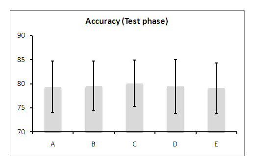
These results can also be contrasted by Friedman and Friedman Aligned procedures. Tables 32 and 33 show the ranks and the p-values achived by each configuration (we also provide figures depicting the ranks achieved in both procedures):
| Using configuration C as control algorithm (Rank: 2.000) | ||||
|---|---|---|---|---|
| Configuration | Rank | Holm | Hochberg | Finner |
| A | 3.250 | 0.00660 | 0.00660 | 0.00439 |
| B | 2.983 | 0.01796 | 0.01601 | 0.01601 |
| D | 3.067 | 0.01796 | 0.01601 | 0.01196 |
| E | 3.700 | 0.00013 | 0.00013 | 0.00013 |
| Using configuration C as control algorithm (Rank: 45.417) | ||||
|---|---|---|---|---|
| Configuration | Rank | Holm | Hochberg | Finner |
| A | 81.533 | 0.00366 | 0.00257 | 0.00244 |
| B | 75.200 | 0.00793 | 0.00793 | 0.00793 |
| D | 81.700 | 0.00366 | 0.00257 | 0.00244 |
| E | 93.650 | 0.00007 | 0.00007 | 0.00007 |
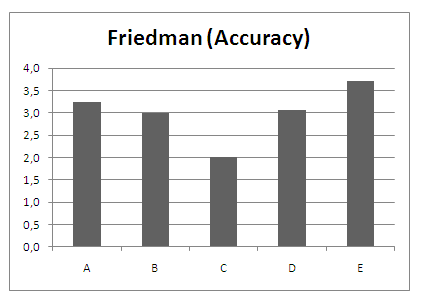
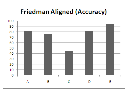
Considering these results, we may conclude that configuration C, 2BLX0.3-4BLX0.5-2BLX0.7, is the best performing from those considered in the study. Its performance is better than the rest of the multiple descendants crossover operator considered, and much better than the performance obtained by not using multiple descendants at all. Thus, these results justify the selection of the crossover operator 2BLX0.3-4BLX0.5-2BLX0.7 to its employment in CIW-NN.
Study of the behavior of CIW-NN as a multiclassifier
The cooperation between the three different populations of CIW-NN can be tuned in several ways. An suitable modification of the fitness function would be to treat the different populations as isolated classifiers, and to obtain the output of the classification process by building a multiclasifier, both in training and test phases.
Thus, an interesting question that arises is to discern which approach is better for CIW-NN: The one originally described for CIW-NN, where IS, FW and IW are applied to the same set of data to build a single classifier, or to apply these techniques to three isolated training sets and to build a multiclassifier, which combines votes of each separate 1-NN classifier by a majority voting process.
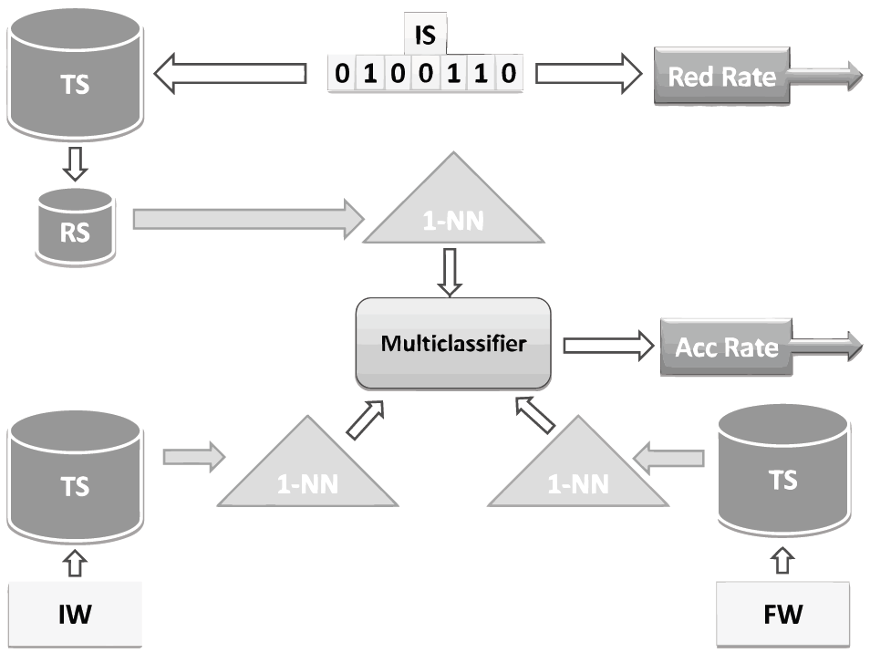
To compare these two approaches, we have carried out an experiment over the 30 small data sets of the general framework. We have considered the accuracy rates obtained in training and test phases, and the time elapsed during the execution of the methods.
The results obtained can be downloaded as an Excel document by clicking on the following link: ![]()
Table 32 shows the average accuracy results achieved in training and test phases, and the time elapsed during its execution (in seconds):
| Basic | Multiclassifier | |||||||||
|---|---|---|---|---|---|---|---|---|---|---|
| Training | Test | - | Training | Test | - | |||||
| Data set | Accuracy | Std. | Accuracy | Std. | Time | Accuracy | Std. | Accuracy | Std. | Time |
| Australian | 85.52 | 1.05 | 81.74 | 3.44 | 63.92 | 83.83 | 1.03 | 82.15 | 3.75 | 212.62 |
| Balance | 83.64 | 1.05 | 85.75 | 4.13 | 37.34 | 83.48 | 1.03 | 85.63 | 3.98 | 100.79 |
| Bands | 71.14 | 1.82 | 75.52 | 5.57 | 64.50 | 71.05 | 1.82 | 75.87 | 5.87 | 158.84 |
| Breast | 76.30 | 1.57 | 70.62 | 7.44 | 7.36 | 77.51 | 1.54 | 70.24 | 7.43 | 28.06 |
| Bupa | 71.57 | 2.79 | 60.95 | 7.50 | 10.24 | 67.03 | 2.77 | 61.11 | 7.71 | 35.08 |
| Car | 88.58 | 2.01 | 95.89 | 1.17 | 440.59 | 88.61 | 2.04 | 95.54 | 1.10 | 923.85 |
| Cleveland | 61.64 | 1.85 | 56.43 | 5.54 | 9.16 | 62.58 | 1.85 | 57.02 | 5.31 | 38.13 |
| Contraceptive | 48.04 | 1.28 | 45.22 | 2.59 | 481.18 | 46.90 | 1.26 | 45.57 | 2.62 | 855.38 |
| Dermatology | 96.02 | 1.50 | 96.72 | 3.17 | 34.60 | 96.16 | 1.49 | 96.52 | 2.93 | 105.45 |
| German | 72.16 | 1.25 | 72.10 | 2.51 | 299.23 | 73.46 | 1.24 | 71.96 | 2.75 | 555.39 |
| Glass | 68.91 | 1.93 | 75.72 | 11.13 | 5.47 | 68.23 | 1.89 | 72.53 | 10.42 | 17.57 |
| Hayes-roth | 78.11 | 1.62 | 72.15 | 12.73 | 3.59 | 77.09 | 1.64 | 72.06 | 11.89 | 6.24 |
| Housevotes | 96.02 | 1.12 | 94.93 | 4.12 | 34.05 | 95.24 | 1.14 | 95.04 | 4.29 | 90.39 |
| Iris | 96.00 | 0.82 | 93.33 | 5.96 | 3.68 | 97.62 | 0.82 | 94.00 | 5.89 | 7.36 |
| Lymphography | 85.67 | 2.44 | 79.30 | 12.22 | 3.45 | 85.67 | 2.48 | 79.67 | 12.57 | 11.82 |
| Monk-2 | 88.45 | 2.08 | 100.00 | 0.00 | 26.79 | 86.37 | 2.06 | 100.00 | 0.00 | 59.83 |
| Movement | 96.13 | 1.37 | 83.06 | 3.32 | 57.23 | 97.27 | 1.34 | 83.62 | 3.09 | 232.22 |
| New Thyroid | 72.82 | 1.53 | 95.82 | 3.15 | 6.75 | 72.20 | 1.57 | 96.25 | 3.05 | 16.33 |
| Pima | 73.38 | 1.01 | 71.24 | 2.03 | 105.56 | 72.00 | 0.99 | 71.43 | 1.84 | 204.57 |
| Saheart | 79.91 | 1.57 | 65.37 | 5.33 | 22.16 | 81.63 | 1.55 | 64.90 | 4.98 | 74.93 |
| Sonar | 82.98 | 2.87 | 87.00 | 3.38 | 18.46 | 82.83 | 2.91 | 87.31 | 3.35 | 52.94 |
| Spectfheart | 55.19 | 2.84 | 77.92 | 13.60 | 17.89 | 56.53 | 2.89 | 77.62 | 13.29 | 69.51 |
| Tae | 75.84 | 0.91 | 65.71 | 3.26 | 3.93 | 75.22 | 0.89 | 66.83 | 3.20 | 8.19 |
| Tic-tac-toe | 66.07 | 2.06 | 87.37 | 3.34 | 134.31 | 65.94 | 2.06 | 87.44 | 3.64 | 328.54 |
| Vehicle | 72.44 | 1.12 | 71.28 | 0.79 | 123.21 | 73.01 | 1.13 | 71.69 | 0.82 | 346.27 |
| Vowel | 97.50 | 0.84 | 98.28 | 3.78 | 303.91 | 98.44 | 0.83 | 98.12 | 3.54 | 468.36 |
| Wine | 96.71 | 0.60 | 97.16 | 2.46 | 5.61 | 95.03 | 0.61 | 96.51 | 2.41 | 14.13 |
| Wisconsin | 52.17 | 1.43 | 96.00 | 2.84 | 86.64 | 52.98 | 1.42 | 96.89 | 2.79 | 183.71 |
| Yeast | 90.69 | 2.84 | 52.76 | 3.89 | 487.48 | 91.12 | 2.85 | 53.08 | 3.54 | 796.89 |
| Zoo | 61.48 | 2.04 | 97.50 | 3.61 | 3.80 | 61.24 | 2.07 | 97.28 | 3.66 | 6.77 |
| Average | 78.04 | 1.64 | 80.09 | 4.80 | 96.74 | 77.88 | 1.64 | 80.13 | 4.72 | 200.34 |
To contrast these results, we perform a Wilcoxon Signed Ranks test (see the SCI2S Thematic Public Website on Statistical Inference in Computational Intelligence and Data Mining for detailed information about this 1x1 non-parametric statistical test ) with the accuracy results on test phase.
Table 33 reports the results achieved:
| Comparison | R + | R - | P-value |
|---|---|---|---|
| Basic VS Multiclassifier | 156.5 | 278.5 | 0.19375 |
The results obtained in this experiment allow us to conclude the following facts:
- The multiclassifier approach slightly improves the results achieved by the basic definition of CIW-NN. However, this improvement is not enough to manifest significant differences between them, when the results are contrasted with a Wilcoxon test. The p-value obtained (0.19375) is higher than any typical level of significance used in statistics, so the hypothesis of equality cannot be rejected.
- The time consumption of the basic approach is more than two times lower than that of the multiclassifier. This new scheme involves the execution of three 1-NN classification processes each time the fitness function needs to be computed. Although most of the classification results can be cached to ease this drawback, two of these 1-NN classifiers (those related to FW and IW populations) must work with the complete training set, instead of just using a reduced set as the basic approach does.
These two facts, along with the necessity of keeping three training sets in the test classification phase (instead of one), allows us to reject the proposition of employing a multiclassifier in CIW-NN, since the small improvement in accuracy is not enough to justify the increase in complexity of the algorithm, either in execution time or in memory requirements.
Adjustment of the epoch lenght in FW and IW populations
Another issue concerning the set up of CIW-NN is the concrete number of evaluations defined for each epoch of FW and IW populations. The length of each epoch must be enough wide to allow the crossover operator to show a suitable behaviour, enhancing the convergence power of CIW-NN.
Since a crossover operator with 8 descendants have been selected (see Section 4.2.1), the length of the epoch must be a whole multiple of 8. Table 34 summarizes the 4 configurations tested. All of them ranges for a low number of generations/epoch to a wide number (20 generations).
| Code | Epoch length | Generations/Epoch |
|---|---|---|
| Epoch 8 | 8 | 1 |
| Epoch 40 | 40 | 5 |
| Epoch 80 | 80 | 10 |
| Epoch 160 | 160 | 20 |
We have carried out an experiment on the 30 small data sets of the general framework. Due to this issue only affecting the dynamics of the IW and FW populations, we will only take into consideration in this comparison the accuracy obtained, since it is the measure which composes their fitness functions.
The results obtained can be downloaded as an Excel document by clicking on the following link: ![]()
Tables 35 and 36 shows the average accuracy results achieved in training and test phase, respectively:
| Configuration | Epoch 8 | Epoch 40 | Epoch 80 | Epoch 160 | ||||
|---|---|---|---|---|---|---|---|---|
| Dataset | Accuracy | Std. Dev | Accuracy | Std. Dev | Accuracy | Std. Dev | Accuracy | Std. Dev |
| Australian | 84.80 | 0.64 | 85.52 | 1.05 | 84.28 | 1.05 | 83.38 | 1.29 |
| Balance | 83.99 | 1.50 | 83.64 | 1.05 | 83.46 | 1.61 | 83.84 | 0.93 |
| Bands | 71.57 | 1.20 | 71.14 | 1.82 | 70.91 | 1.55 | 71.24 | 2.60 |
| Breast | 74.38 | 1.55 | 76.30 | 1.57 | 73.43 | 1.78 | 72.73 | 2.02 |
| Bupa | 68.79 | 3.13 | 71.57 | 2.79 | 66.91 | 2.54 | 67.45 | 2.15 |
| Car | 86.91 | 1.09 | 88.58 | 2.01 | 89.89 | 0.84 | 90.15 | 0.98 |
| Cleveland | 60.38 | 1.56 | 61.64 | 1.85 | 60.59 | 1.98 | 59.68 | 2.33 |
| Contraceptive | 49.31 | 1.35 | 48.04 | 1.28 | 47.20 | 0.70 | 47.33 | 1.62 |
| Dermatology | 95.97 | 1.58 | 96.02 | 1.50 | 95.80 | 1.60 | 96.22 | 1.34 |
| German | 72.92 | 1.12 | 72.16 | 1.25 | 71.29 | 0.94 | 72.19 | 1.32 |
| Glass | 70.18 | 3.60 | 68.91 | 1.93 | 70.68 | 4.14 | 71.56 | 2.41 |
| Hayes-roth | 77.37 | 3.98 | 78.11 | 1.62 | 78.28 | 1.95 | 77.19 | 2.55 |
| Housevotes | 94.60 | 0.55 | 96.02 | 1.12 | 94.39 | 0.78 | 95.03 | 1.15 |
| Iris | 94.89 | 1.23 | 96.00 | 0.82 | 96.61 | 1.02 | 95.57 | 1.00 |
| Lymphography | 82.92 | 3.15 | 85.67 | 2.44 | 82.24 | 2.71 | 81.64 | 3.06 |
| Monk-2 | 83.95 | 3.50 | 88.45 | 2.08 | 87.11 | 6.98 | 86.77 | 5.09 |
| Movement | 68.65 | 1.61 | 61.48 | 1.37 | 67.28 | 2.52 | 67.77 | 2.64 |
| New Thyroid | 93.97 | 1.20 | 96.13 | 1.53 | 93.30 | 1.79 | 93.92 | 0.94 |
| Pima | 75.04 | 1.22 | 72.82 | 1.01 | 72.05 | 0.77 | 72.29 | 1.37 |
| Saheart | 72.53 | 1.04 | 73.38 | 1.57 | 69.37 | 2.72 | 69.10 | 2.38 |
| Sonar | 81.28 | 2.62 | 79.91 | 2.87 | 81.23 | 2.60 | 80.65 | 2.93 |
| Spectfheart | 82.39 | 2.16 | 82.98 | 2.84 | 80.65 | 1.31 | 79.78 | 1.33 |
| Tae | 56.28 | 3.81 | 55.19 | 0.91 | 55.65 | 1.90 | 55.86 | 2.03 |
| Tic-tac-toe | 75.88 | 1.16 | 75.84 | 2.06 | 78.63 | 1.52 | 80.35 | 2.36 |
| Vehicle | 68.62 | 2.27 | 66.07 | 1.12 | 68.12 | 1.77 | 68.99 | 2.38 |
| Vowel | 77.25 | 2.12 | 72.44 | 0.84 | 80.52 | 2.71 | 81.16 | 1.89 |
| Wine | 96.69 | 1.17 | 97.50 | 0.60 | 96.88 | 1.14 | 96.50 | 1.69 |
| Wisconsin | 95.35 | 0.44 | 96.71 | 1.43 | 95.99 | 0.39 | 95.92 | 0.50 |
| Yeast | 54.69 | 1.25 | 52.17 | 2.84 | 51.56 | 1.62 | 52.70 | 1.37 |
| Zoo | 91.60 | 1.39 | 90.69 | 2.04 | 92.12 | 2.24 | 90.17 | 2.81 |
| Average | 78.10 | 1.81 | 78.04 | 1.64 | 77.88 | 1.91 | 77.90 | 1.95 |
| Configuration | Epoch 8 | Epoch 40 | Epoch 80 | Epoch 160 | ||||
|---|---|---|---|---|---|---|---|---|
| Dataset | Accuracy | Std. Dev | Accuracy | Std. Dev | Accuracy | Std. Dev | Accuracy | Std. Dev |
| Australian | 81.88 | 3.90 | 81.74 | 3.44 | 81.45 | 3.42 | 81.30 | 4.07 |
| Balance | 85.44 | 2.07 | 85.75 | 4.13 | 83.84 | 4.28 | 84.15 | 4.51 |
| Bands | 74.41 | 4.39 | 75.52 | 5.57 | 75.71 | 5.67 | 74.78 | 5.40 |
| Breast | 70.72 | 6.89 | 70.62 | 7.44 | 70.73 | 5.85 | 70.03 | 6.43 |
| Bupa | 65.73 | 8.82 | 60.95 | 7.50 | 60.89 | 4.67 | 62.88 | 6.55 |
| Car | 95.14 | 1.45 | 95.89 | 1.17 | 95.60 | 1.01 | 95.95 | 1.01 |
| Cleveland | 57.09 | 6.35 | 56.43 | 5.54 | 56.45 | 7.79 | 56.77 | 3.62 |
| Contraceptive | 46.03 | 2.34 | 45.22 | 2.59 | 46.30 | 3.31 | 46.44 | 3.41 |
| Dermatology | 96.46 | 3.64 | 96.72 | 3.17 | 94.82 | 3.30 | 94.00 | 4.17 |
| German | 71.60 | 2.29 | 72.10 | 2.51 | 72.40 | 2.69 | 72.60 | 2.91 |
| Glass | 75.16 | 12.32 | 75.72 | 11.13 | 74.23 | 13.05 | 74.63 | 12.25 |
| Hayes-roth | 74.98 | 8.24 | 72.15 | 12.73 | 72.26 | 10.54 | 73.03 | 9.64 |
| Housevotes | 93.54 | 4.38 | 94.93 | 4.12 | 93.32 | 4.55 | 94.70 | 3.87 |
| Iris | 94.00 | 3.59 | 93.33 | 5.96 | 94.00 | 5.54 | 94.67 | 5.81 |
| Lymphography | 75.33 | 11.37 | 79.30 | 12.22 | 79.06 | 12.47 | 79.30 | 9.80 |
| Monk-2 | 96.79 | 6.38 | 100.00 | 0.00 | 100.00 | 0.00 | 99.77 | 0.70 |
| Movement | 84.17 | 4.82 | 83.06 | 3.32 | 84.17 | 4.82 | 84.17 | 4.82 |
| New Thyroid | 96.30 | 2.82 | 95.82 | 3.15 | 96.75 | 3.01 | 95.82 | 2.55 |
| Pima | 69.55 | 3.83 | 71.24 | 2.03 | 71.50 | 4.21 | 71.12 | 5.66 |
| Saheart | 66.22 | 3.76 | 65.37 | 5.33 | 66.02 | 4.52 | 64.28 | 4.27 |
| Sonar | 88.45 | 7.21 | 87.00 | 3.38 | 87.52 | 7.82 | 87.52 | 7.82 |
| Spectfheart | 77.55 | 4.58 | 77.92 | 13.60 | 77.68 | 2.71 | 77.58 | 4.49 |
| Tae | 65.71 | 13.27 | 65.71 | 3.26 | 65.71 | 13.27 | 65.71 | 13.27 |
| Tic-tac-toe | 86.63 | 3.57 | 87.37 | 3.34 | 88.10 | 4.22 | 88.21 | 3.19 |
| Vehicle | 70.22 | 3.67 | 71.28 | 0.79 | 70.81 | 2.92 | 70.58 | 3.02 |
| Vowel | 97.88 | 1.23 | 98.28 | 3.78 | 97.88 | 1.23 | 97.88 | 1.23 |
| Wine | 96.63 | 3.71 | 97.16 | 2.46 | 96.89 | 2.22 | 96.89 | 2.22 |
| Wisconsin | 96.86 | 2.00 | 96.00 | 2.84 | 96.28 | 1.59 | 96.00 | 1.54 |
| Yeast | 51.89 | 4.21 | 52.76 | 3.89 | 51.42 | 3.54 | 52.22 | 2.31 |
| Zoo | 96.00 | 6.29 | 97.50 | 3.61 | 94.89 | 6.46 | 95.17 | 6.26 |
| Average | 79.95 | 5.11 | 80.09 | 4.80 | 79.89 | 5.05 | 79.94 | 4.89 |
The results achieved in test phase can be viewed graphycally. The following picture depicts the average accuracy and standard deviations achieved by each configuration:
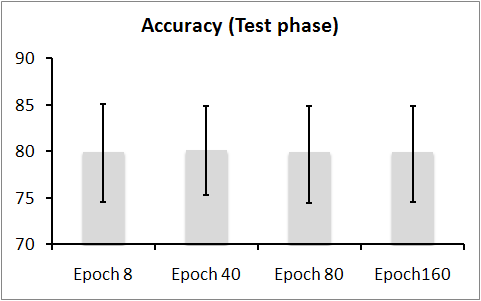
These results can also be contrasted by Friedman and Friedman Aligned procedures. Tables 37 and 38 show the ranks and the p-values achived by each configuration (we also provide figures depicting the ranks achieved in both procedures):
| Using Epoch 40 as control algorithm (Rank: 2.317) | ||||
|---|---|---|---|---|
| Configuration | Rank | Holm | Hochberg | Finner |
| Epoch 8 | 2.600 | 1.18598 | 0.77891 | 0.51569 |
| Epoch 80 | 2.550 | 1.18598 | 0.77891 | 0.51569 |
| Epoch 160 | 2.533 | 1.18598 | 0.77891 | 0.51569 |
| Using Epoch 40 as control algorithm (Rank: 54.217) | ||||
|---|---|---|---|---|
| Configuration | Rank | Holm | Hochberg | Finner |
| Epoch 8 | 61.067 | 0.81103 | 0.61153 | 0.44565 |
| Epoch 80 | 64.117 | 0.81103 | 0.61153 | 0.44565 |
| Epoch 160 | 62.600 | 0.81103 | 0.61153 | 0.44565 |
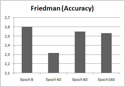
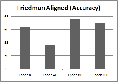
Considering these results, we may conclude that using an epoch length of 40 evaluations may be the best option for CIW-NN in the problems selected. However, it is important to note that CIW-NN is not very sensitive to changes on these parameters, since none of the configurations tested has achieved a significant improvement over the rest.
Setting up the weights of distance function for IW individuals
When describing the effects of the weights computed by the IW population of CIW-NN to the training set, there are stated the following facts:
- Distances computed from instances belonging to classes marked with maximum weights (IWc(X) = 1:0) will be very small (a (1.0 - γ) factor of their former value).
- Distances computed from instances belonging to classes marked with minimum weights (IWc(X) = 0:0) will not change.
- The remaining possible values will modify the distance computed within this range.
This behaviour is controlled by the γ weight used in the CIW-NN distance function:
$$Distance(X,Y)=\gamma · (1.0-IW_{c(X)})·FWDist(X.Y)+(1.0-\gamma ) ·FWDist(X,Y)$$
In this distance function, two terms can be highlighted:
- A fixed term, which is not dependant of the weights of the IW population.
- A variable term, which is dependant of the weights of the IW population.
By default, CIW-NN uses γ = 0.8. However, it may be interesting to analyze the impact of changes in this value to the global behaviour of CIW-NN.
To do so, we have defined several configurations for setting up the weights of distance function of CIW-NN. Table 39 summarizes them:
| Code | γ weight (weight of the variable term) |
|---|---|
| A | 1.00 |
| B | 0.80 |
| C | 0.67 |
| D | 0.50 |
We have carried out an experiment on the 30 small data sets of the general framework. Due to this issue only affecting the dynamics of the IW population, we will only take into consideration in this comparison the accuracy obtained, since it is the measure which composes their fitness functions.
The results obtained can be downloaded as an Excel document by clicking on the following link: ![]()
Tables 40 and 41 shows the average accuracy results achieved in training and test phase, respectively:
| Configuration | A | B | C | D | ||||
|---|---|---|---|---|---|---|---|---|
| Dataset | Accuracy | Std. Dev | Accuracy | Std. Dev | Accuracy | Std. Dev | Accuracy | Std. Dev |
| Australian | 84.80 | 0.84 | 85.52 | 1.05 | 84.69 | 0.74 | 86.25 | 0.70 |
| Balance | 81.86 | 2.43 | 83.64 | 1.05 | 79.85 | 2.69 | 83.31 | 2.87 |
| Bands | 70.25 | 2.51 | 71.14 | 1.82 | 72.38 | 2.04 | 71.70 | 2.02 |
| Breast | 74.46 | 1.90 | 76.30 | 1.57 | 76.16 | 1.66 | 75.91 | 1.53 |
| Bupa | 70.66 | 2.15 | 71.57 | 2.79 | 72.50 | 2.37 | 72.11 | 2.42 |
| Car | 88.43 | 0.69 | 88.58 | 2.01 | 87.95 | 0.73 | 89.88 | 0.73 |
| Cleveland | 61.04 | 1.96 | 61.64 | 1.85 | 61.70 | 1.49 | 62.49 | 1.58 |
| Contraceptive | 46.55 | 1.19 | 48.04 | 1.28 | 49.61 | 1.37 | 48.00 | 1.27 |
| Dermatology | 95.64 | 1.16 | 96.02 | 1.50 | 93.07 | 1.05 | 97.09 | 1.08 |
| German | 70.84 | 1.92 | 72.16 | 1.25 | 69.67 | 1.60 | 72.29 | 1.65 |
| Glass | 69.78 | 3.74 | 68.91 | 1.93 | 70.13 | 2.17 | 71.23 | 4.19 |
| Hayes-roth | 77.68 | 1.79 | 78.11 | 1.62 | 76.46 | 1.57 | 79.13 | 1.60 |
| Housevotes | 94.34 | 1.10 | 96.02 | 1.12 | 99.52 | 1.09 | 95.79 | 1.13 |
| Iris | 95.44 | 0.64 | 96.00 | 0.82 | 92.41 | 0.71 | 96.89 | 0.65 |
| Lymphography | 82.86 | 2.82 | 85.67 | 2.44 | 84.51 | 3.39 | 84.31 | 3.13 |
| Monk-2 | 83.40 | 8.10 | 88.45 | 2.08 | 85.41 | 6.29 | 84.85 | 6.97 |
| Movement | 66.85 | 1.70 | 61.48 | 1.37 | 64.99 | 1.69 | 68.30 | 1.57 |
| New Thyroid | 93.69 | 1.48 | 96.13 | 1.53 | 92.14 | 1.91 | 95.14 | 1.82 |
| Pima | 71.94 | 2.80 | 72.82 | 1.01 | 74.00 | 2.49 | 73.39 | 2.28 |
| Saheart | 71.04 | 1.84 | 73.38 | 1.57 | 73.71 | 2.12 | 72.49 | 2.10 |
| Sonar | 80.98 | 1.75 | 79.91 | 2.87 | 82.94 | 2.23 | 82.43 | 2.24 |
| Spectfheart | 81.45 | 1.16 | 82.98 | 2.84 | 82.63 | 1.00 | 82.90 | 1.10 |
| Tae | 54.48 | 3.28 | 55.19 | 0.91 | 56.17 | 2.73 | 55.93 | 2.68 |
| Tic-tac-toe | 76.34 | 1.82 | 75.84 | 2.06 | 80.29 | 2.00 | 77.79 | 1.93 |
| Vehicle | 67.29 | 2.14 | 66.07 | 1.12 | 68.95 | 1.98 | 68.74 | 1.83 |
| Vowel | 78.01 | 2.93 | 72.44 | 0.84 | 81.00 | 2.33 | 79.46 | 2.35 |
| Wine | 96.30 | 0.89 | 97.50 | 0.60 | 95.07 | 1.12 | 97.75 | 1.16 |
| Wisconsin | 95.15 | 0.45 | 96.71 | 1.43 | 92.97 | 0.42 | 96.60 | 0.38 |
| Yeast | 51.40 | 1.63 | 52.17 | 2.84 | 54.08 | 1.92 | 52.85 | 1.82 |
| Zoo | 91.03 | 2.57 | 90.69 | 2.04 | 92.96 | 2.38 | 92.48 | 2.38 |
| Average | 77.47 | 2.05 | 78.04 | 1.64 | 78.26 | 1.91 | 78.92 | 1.97 |
| Configuration | A | B | C | D | ||||
|---|---|---|---|---|---|---|---|---|
| Dataset | Accuracy | Std. Dev | Accuracy | Std. Dev | Accuracy | Std. Dev | Accuracy | Std. Dev |
| Australian | 80.00 | 4.62 | 81.74 | 3.44 | 80.87 | 4.29 | 81.74 | 3.73 |
| Balance | 84.15 | 4.59 | 85.75 | 4.13 | 84.47 | 4.62 | 84.80 | 4.57 |
| Bands | 73.11 | 3.86 | 75.52 | 5.57 | 74.41 | 4.31 | 74.97 | 4.02 |
| Breast | 70.64 | 4.90 | 70.62 | 7.44 | 71.68 | 6.32 | 69.22 | 7.85 |
| Bupa | 63.12 | 8.07 | 60.95 | 7.50 | 63.99 | 6.31 | 63.43 | 5.91 |
| Car | 95.77 | 1.32 | 95.89 | 1.17 | 95.77 | 1.32 | 95.77 | 1.32 |
| Cleveland | 57.75 | 4.41 | 56.43 | 5.54 | 56.74 | 5.74 | 56.43 | 5.49 |
| Contraceptive | 45.28 | 2.54 | 45.22 | 2.59 | 44.88 | 3.64 | 44.61 | 3.66 |
| Dermatology | 96.19 | 3.25 | 96.72 | 3.17 | 96.19 | 3.86 | 96.19 | 3.86 |
| German | 70.60 | 2.06 | 72.10 | 2.51 | 71.10 | 3.27 | 70.80 | 3.28 |
| Glass | 73.17 | 12.29 | 75.72 | 11.13 | 77.33 | 12.76 | 76.99 | 11.45 |
| Hayes-roth | 74.41 | 10.39 | 72.15 | 12.73 | 71.98 | 12.22 | 70.49 | 12.37 |
| Housevotes | 93.07 | 4.42 | 94.93 | 4.12 | 93.30 | 4.35 | 93.53 | 4.40 |
| Iris | 94.00 | 4.67 | 93.33 | 5.96 | 94.00 | 5.54 | 94.67 | 4.99 |
| Lymphography | 75.34 | 14.12 | 79.30 | 12.22 | 78.68 | 10.40 | 77.96 | 9.61 |
| Monk-2 | 99.54 | 0.92 | 100.00 | 0.00 | 99.77 | 0.70 | 99.77 | 0.70 |
| Movement | 78.89 | 4.84 | 83.06 | 3.32 | 86.11 | 5.69 | 87.22 | 5.85 |
| New Thyroid | 95.37 | 3.58 | 95.82 | 3.15 | 96.75 | 3.01 | 96.75 | 3.01 |
| Pima | 68.12 | 5.04 | 71.24 | 2.03 | 69.43 | 5.05 | 69.56 | 5.20 |
| Saheart | 64.72 | 5.75 | 65.37 | 5.33 | 63.84 | 5.11 | 63.41 | 5.22 |
| Sonar | 85.57 | 7.41 | 87.00 | 3.38 | 87.52 | 6.80 | 87.05 | 7.38 |
| Spectfheart | 77.59 | 9.12 | 77.92 | 13.60 | 74.94 | 8.02 | 75.67 | 8.45 |
| Tae | 65.04 | 11.97 | 65.71 | 3.26 | 65.04 | 13.03 | 64.38 | 12.76 |
| Tic-tac-toe | 87.47 | 4.72 | 87.37 | 3.34 | 87.78 | 4.86 | 87.88 | 4.95 |
| Vehicle | 70.22 | 2.56 | 71.28 | 0.79 | 71.52 | 4.07 | 71.04 | 3.73 |
| Vowel | 96.16 | 1.41 | 98.28 | 3.78 | 98.48 | 1.22 | 98.79 | 0.88 |
| Wine | 93.24 | 6.15 | 97.16 | 2.46 | 96.08 | 4.35 | 95.49 | 4.18 |
| Wisconsin | 96.42 | 1.94 | 96.00 | 2.84 | 96.00 | 1.66 | 95.57 | 1.85 |
| Yeast | 51.35 | 3.50 | 52.76 | 3.89 | 52.16 | 4.01 | 52.29 | 3.93 |
| Zoo | 96.00 | 6.29 | 97.50 | 3.61 | 96.00 | 6.29 | 96.00 | 6.29 |
| Average | 79.08 | 5.36 | 80.09 | 4.80 | 79.89 | 5.43 | 79.75 | 5.36 |
The results achieved in test phase can be viewed graphycally. The following picture depicts the average accuracy and standard deviations achieved by each configuration:
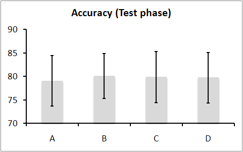
These results can also be contrasted by Friedman and Friedman Aligned procedures. Tables 42 and 43 show the ranks and the p-values achived by each configuration (we also provide figures depicting the ranks achieved in both procedures):
| Using configuration B as control algorithm (Rank: 1.950) | ||||
|---|---|---|---|---|
| Configuration | Rank | Holm | Hochberg | Finner |
| A | 3.133 | 0.00116 | 0.00116 | 0.00116 |
| C | 2.350 | 0.23014 | 0.23014 | 0.23014 |
| D | 2.567 | 0.12863 | 0.12863 | 0.09490 |
| Using configuration B as control algorithm (Rank: 44.033) | ||||
|---|---|---|---|---|
| Configuration | Rank | Holm | Hochberg | Finner |
| A | 79.633 | 0.000221 | 0.000221 | 0.000221 |
| C | 56.233 | 0.174352 | 0.174352 | 0.174352 |
| D | 62.100 | 0.088535 | 0.088535 | 0.065661 |
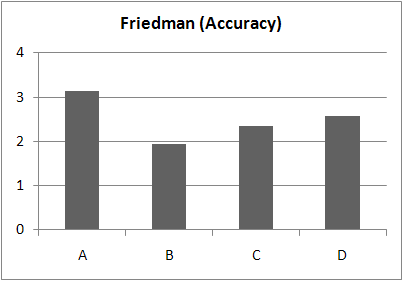
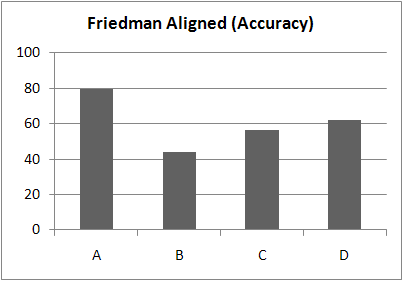
Considering these results, we may conclude that the configuration B (the one selected by default) is the best option for CIW-NN. Higher weights for the fixed term may led to a diminish of the modeling capabilities of the IW population, thus decreasing slightly the performance of the model. In contrast, disabling the fixed term (setting its weight to 0, configuration A) may led to a unstable behaviour in some domains, making harder for the IW population to find a suitable set of weights. This fact is contrasted by the statistical comparison performed, where configuration A is strongly improved by configuration B, with a very low p-value (0.00116 or less).
Determining the optimum value for the k parameter
Finding an optimal value for the k parameter turns out to be an interesting question when using k-NN based classifiers, such as CIW-NN. In this experiment, our aim is to determine the behavior of CIW-NN when the k value id modified, as well as establishing an optimal value which suits best in most cases. The classifier will obtain smoother class boundaries as the k value is increased (even smoother than when using only an Instance Selection algorithm), but it may significantly decrease the accuracy of the classifier.
To do so, we have selected the set {1,3,5,7,9} as possible values for k. We have carried out an experiment on the 30 small data sets of the general framework. Average accuracy in training and test phases have been considered as performance criteria.
The results obtained can be downloaded as an Excel document by clicking on the following link: ![]()
Tables 44 and 45 shows the average accuracy results achieved in training and test phase, respectively:
| Configuration | 1-NN | 3-NN | 5-NN | 7-NN | 9-NN | |||||
|---|---|---|---|---|---|---|---|---|---|---|
| Dataset | Accuracy | Std. Dev | Accuracy | Std. Dev | Accuracy | Std. Dev | Accuracy | Std. Dev | Accuracy | Std. Dev |
| Australian | 85.52 | 1.05 | 85.91 | 0.75 | 85.68 | 0.37 | 85.14 | 1.42 | 85.72 | 0.73 |
| Balance | 83.64 | 1.05 | 85.05 | 1.68 | 84.57 | 1.86 | 85.58 | 1.06 | 85.60 | 1.46 |
| Bands | 71.14 | 1.82 | 70.07 | 1.44 | 69.37 | 1.17 | 69.33 | 1.57 | 69.22 | 1.85 |
| Breast | 76.30 | 1.57 | 75.72 | 1.78 | 75.52 | 1.92 | 74.35 | 3.49 | 73.35 | 3.24 |
| Bupa | 71.57 | 2.79 | 68.89 | 2.68 | 67.34 | 2.60 | 68.34 | 2.93 | 67.95 | 5.58 |
| Car | 88.58 | 2.01 | 86.44 | 2.11 | 85.92 | 2.31 | 86.65 | 2.24 | 88.37 | 2.37 |
| Cleveland | 61.64 | 1.85 | 60.62 | 1.50 | 60.69 | 1.53 | 61.39 | 1.89 | 60.43 | 1.31 |
| Contraceptive | 48.04 | 1.28 | 48.32 | 1.46 | 48.74 | 1.47 | 48.92 | 2.26 | 48.77 | 1.52 |
| Dermatology | 96.02 | 1.50 | 96.36 | 1.97 | 95.42 | 1.37 | 95.26 | 1.65 | 95.87 | 1.94 |
| German | 72.16 | 1.25 | 72.51 | 2.08 | 72.59 | 1.08 | 72.54 | 1.26 | 72.61 | 0.64 |
| Glass | 68.91 | 1.93 | 68.20 | 5.61 | 68.56 | 2.78 | 68.06 | 3.31 | 68.19 | 4.19 |
| Hayes-roth | 78.11 | 1.62 | 68.01 | 4.73 | 65.18 | 4.27 | 68.21 | 5.24 | 68.82 | 4.59 |
| Housevotes | 96.02 | 1.12 | 95.58 | 1.09 | 95.86 | 1.03 | 95.17 | 1.07 | 95.63 | 1.13 |
| Iris | 96.00 | 0.82 | 96.74 | 1.11 | 96.44 | 1.19 | 95.26 | 1.73 | 95.85 | 1.73 |
| Lymphography | 85.67 | 2.44 | 85.20 | 3.11 | 83.64 | 2.67 | 82.66 | 3.33 | 84.91 | 4.06 |
| Monk-2 | 88.45 | 2.08 | 87.53 | 3.38 | 86.00 | 6.74 | 85.21 | 4.22 | 86.21 | 6.83 |
| Movement | 61.48 | 1.37 | 63.95 | 4.03 | 60.46 | 3.54 | 60.99 | 3.78 | 60.40 | 4.89 |
| New Thyroid | 96.13 | 1.53 | 95.76 | 1.25 | 95.61 | 1.11 | 96.79 | 1.76 | 95.92 | 1.19 |
| Pima | 72.82 | 1.01 | 74.03 | 1.72 | 75.45 | 1.43 | 75.54 | 0.91 | 75.62 | 0.78 |
| Saheart | 73.38 | 1.57 | 73.71 | 0.95 | 73.28 | 1.16 | 73.30 | 0.94 | 72.49 | 0.95 |
| Sonar | 79.91 | 2.87 | 76.28 | 3.66 | 75.00 | 2.11 | 75.54 | 5.49 | 77.08 | 4.41 |
| Spectfheart | 82.98 | 2.84 | 80.02 | 1.19 | 79.40 | 0.18 | 79.40 | 0.18 | 79.40 | 0.18 |
| Tae | 55.19 | 0.91 | 56.37 | 3.09 | 56.52 | 2.66 | 56.74 | 3.34 | 54.74 | 4.69 |
| Tic-Tac-Toe | 75.84 | 2.06 | 73.89 | 1.71 | 67.62 | 3.03 | 69.28 | 2.16 | 69.35 | 4.45 |
| Vehicle | 66.07 | 1.12 | 65.44 | 2.51 | 65.70 | 1.60 | 66.70 | 1.59 | 66.01 | 2.58 |
| Vowel | 72.44 | 0.84 | 76.25 | 3.68 | 74.47 | 1.90 | 70.38 | 3.76 | 70.75 | 2.62 |
| Wine | 97.50 | 0.60 | 97.75 | 1.28 | 98.06 | 1.59 | 97.57 | 1.13 | 97.19 | 0.98 |
| Wisconsin | 96.71 | 1.43 | 96.52 | 0.63 | 96.34 | 0.58 | 96.12 | 0.59 | 96.07 | 0.78 |
| Yeast | 52.17 | 2.84 | 54.48 | 1.44 | 56.12 | 1.17 | 54.72 | 1.57 | 55.03 | 1.96 |
| Zoo | 90.69 | 2.04 | 90.03 | 3.29 | 90.64 | 5.46 | 91.22 | 3.81 | 91.50 | 7.16 |
| Average | 78.04 | 1.64 | 77.52 | 2.23 | 76.87 | 2.06 | 76.88 | 2.32 | 76.97 | 2.69 |
| Configuration | 1-NN | 3-NN | 5-NN | 7-NN | 9-NN | |||||
|---|---|---|---|---|---|---|---|---|---|---|
| Dataset | Accuracy | Std. Dev | Accuracy | Std. Dev | Accuracy | Std. Dev | Accuracy | Std. Dev | Accuracy | Std. Dev |
| Australian | 81.74 | 3.44 | 84.06 | 5.06 | 84.78 | 4.26 | 84.93 | 3.90 | 84.78 | 2.92 |
| Balance | 85.75 | 4.13 | 86.08 | 2.82 | 86.70 | 3.78 | 87.03 | 3.11 | 88.64 | 3.04 |
| Bands | 75.52 | 5.57 | 74.97 | 7.62 | 74.42 | 7.68 | 75.52 | 5.69 | 71.64 | 7.81 |
| Breast | 70.62 | 7.44 | 69.20 | 3.55 | 70.06 | 6.75 | 72.32 | 8.24 | 71.00 | 6.02 |
| Bupa | 60.95 | 7.50 | 65.37 | 8.72 | 67.56 | 7.92 | 65.64 | 8.99 | 63.33 | 8.20 |
| Car | 95.89 | 1.17 | 94.73 | 1.02 | 89.29 | 2.75 | 91.08 | 3.60 | 95.31 | 2.18 |
| Cleveland | 56.43 | 5.54 | 54.09 | 8.52 | 59.08 | 7.15 | 56.77 | 6.38 | 56.13 | 7.53 |
| Contraceptive | 45.22 | 2.59 | 46.57 | 3.17 | 47.53 | 4.91 | 47.59 | 2.82 | 50.04 | 5.05 |
| Dermatology | 96.72 | 3.17 | 96.73 | 2.66 | 96.46 | 2.42 | 95.09 | 2.92 | 96.16 | 2.80 |
| German | 72.10 | 2.51 | 72.70 | 3.26 | 70.90 | 2.17 | 72.30 | 3.95 | 73.00 | 4.05 |
| Glass | 75.72 | 11.13 | 73.00 | 11.00 | 68.94 | 9.99 | 68.89 | 13.12 | 68.12 | 9.86 |
| Hayes-roth | 72.15 | 12.73 | 70.67 | 11.12 | 69.01 | 12.68 | 76.23 | 10.64 | 70.46 | 12.17 |
| Housevotes | 94.93 | 4.12 | 94.69 | 4.30 | 96.07 | 3.30 | 95.38 | 3.89 | 95.85 | 4.72 |
| Iris | 93.33 | 5.96 | 93.33 | 4.22 | 95.33 | 3.06 | 94.67 | 5.81 | 95.33 | 4.27 |
| Lymphography | 79.30 | 12.22 | 75.20 | 11.99 | 74.58 | 12.92 | 78.77 | 12.60 | 78.01 | 9.48 |
| Monk-2 | 100.00 | 0.00 | 99.32 | 2.05 | 97.92 | 2.19 | 97.50 | 2.77 | 94.23 | 4.79 |
| Movement | 83.06 | 3.32 | 79.17 | 3.61 | 78.78 | 3.72 | 78.94 | 3.59 | 76.17 | 4.55 |
| New Thyroid | 95.82 | 3.15 | 95.35 | 4.21 | 96.30 | 2.75 | 94.89 | 4.42 | 96.77 | 3.57 |
| Pima | 71.24 | 2.03 | 72.81 | 5.17 | 74.49 | 2.71 | 73.19 | 4.09 | 74.74 | 3.51 |
| Saheart | 65.37 | 5.33 | 64.50 | 5.01 | 65.58 | 4.71 | 66.88 | 4.76 | 68.19 | 3.31 |
| Sonar | 87.00 | 3.38 | 84.07 | 9.82 | 82.60 | 10.85 | 79.76 | 8.43 | 74.88 | 8.75 |
| Spectfheart | 77.92 | 13.60 | 77.54 | 6.73 | 74.56 | 5.20 | 76.44 | 7.82 | 76.08 | 7.94 |
| Tae | 65.71 | 3.26 | 65.75 | 10.69 | 65.83 | 11.24 | 65.75 | 9.57 | 65.42 | 8.63 |
| Tic-tac-toe | 87.37 | 3.34 | 84.45 | 2.83 | 76.21 | 4.72 | 78.61 | 1.83 | 78.71 | 1.73 |
| Vehicle | 71.28 | 0.79 | 69.04 | 2.35 | 68.80 | 4.62 | 69.26 | 3.78 | 70.45 | 3.78 |
| Vowel | 98.28 | 3.78 | 97.81 | 2.69 | 97.88 | 3.47 | 96.87 | 3.76 | 95.82 | 4.96 |
| Wine | 97.16 | 2.46 | 98.27 | 3.73 | 97.75 | 2.76 | 96.60 | 3.73 | 96.08 | 3.57 |
| Wisconsin | 96.00 | 2.84 | 96.43 | 2.73 | 96.42 | 3.08 | 97.14 | 2.78 | 95.85 | 2.26 |
| Yeast | 52.76 | 3.89 | 53.17 | 4.56 | 55.80 | 2.37 | 57.42 | 2.86 | 54.45 | 2.70 |
| Zoo | 97.50 | 3.61 | 93.64 | 6.89 | 93.28 | 6.24 | 93.64 | 6.90 | 93.78 | 6.83 |
| Average | 80.09 | 4.80 | 79.42 | 5.40 | 79.10 | 5.41 | 79.50 | 5.56 | 78.98 | 5.37 |
The results achieved in test phase can be viewed graphycally. The following picture depicts the average accuracy and standard deviations achieved by each configuration:
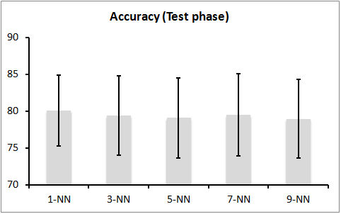
These results can also be contrasted by Friedman and Friedman Aligned procedures. Tables 46 and 47 show the ranks and the p-values achived by each configuration (we also provide figures depicting the ranks achieved in both procedures):
| Using k parameter as 1(1-NN) as control algorithm (Rank: 2.767) | ||||
|---|---|---|---|---|
| Configuration | Rank | Holm | Hochberg | Finner |
| 3-NN | 3.183 | 1.000000 | 0.738215 | 0.769938 |
| 5-NN | 3.133 | 1.000000 | 0.738215 | 0.769938 |
| 7-NN | 2.783 | 1.000000 | 0.967436 | 0.967436 |
| 9-NN | 3.133 | 1.000000 | 0.738215 | 0.769938 |
| Using k parameter as 1(1-NN) as control algorithm (Rank: 65.533) | ||||
|---|---|---|---|---|
| Configuration | Rank | Holm | Hochberg | Finner |
| 3-NN | 76.717 | 0.642597 | 0.447717 | 0.474774 |
| 5-NN | 79.467 | 0.642597 | 0.447717 | 0.474774 |
| 7-NN | 74.050 | 0.642597 | 0.447717 | 0.474774 |
| 9-NN | 81.733 | 0.594769 | 0.447717 | 0.474774 |
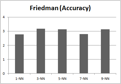
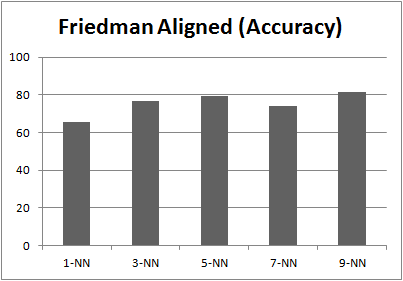
Considering these results, we may conclude that CIW-NN is not too sensitive to the choice of the k parameter for the k-NN classifier. Both Friedman and Friedman Aligned tests do not find significant differences when selecting different numbers of neighbors. Since the accuracy of CIW-NN is sligthly dimished as the k value growths, and its computational requeriments are increased (note that the more neighbors the k-NN rule has to find, the more costly the fitness function will be), we recommend the use of k=1 as the optimum value for CIW-NN.