
Supplementary Material - Artificial Intelligence in Medicine
This website contains supplementary material to the paper:
A. Torres-Martos, A. Anguita-Ruiz, M. Bustos-Aibar, A. Ramírez-Mena, M. Arteaga, G. Bueno, R. Leis, C.M. Aguilera, R. Alcalá, J. Alcalá-Fdez. Multiomics and eXplainable artificial intelligence for decision support in insulin resistance early diagnosis: A pediatric population-based longitudinal study. Artificial Intelligence in Medicine 156 (2024) 102962. doi: 10.1016/j.artmed.2024.102962
Summary:
- Datasets
- Performance measures
- Resampling methods
- Predictive methods analyzed
- Results
- Explainability
- Functional analysis and pathways
- References
Datasets
The variables from the different datasets used in this work are included for the purpose of future replication (see Table S1). The Materials and Methods section of the original manuscript provides a more detailed description of the methodology used to obtain the different data layers.
| Gen | Epi | Clin |
|---|---|---|
| rs683135_A | cg09954592 | origin |
| rs10493846_T | cg04610178 | sex |
| rs2125421_T | cg22699462 | age_years |
| rs10923931_T | cg03161621 | bmi_zscore |
| rs9425291_A | cg22006088 | sistolic_blood_pressure_mm_hg |
| rs234668_G | cg18522464 | distolic_blood_pressure_mm_hg |
| rs4846565_A | cg01183586 | waist_circumference_cm |
| rs7578597_C | cg19194924 | waist_to_height_ratio |
| rs2249105_G | cg16887640 | glucose_mg_dl |
| rs3218878_A | cg23391907 | insulin_mu_l |
| rs3218883_A | cg16740586_ABCG1 | quantitative_insulin_sensitivity_check_index |
| rs3218885_G | cg20075442_ABCG1 | homeostasis_model_assessment |
| rs3218888_C | cg03565996_ABCG1 | leptin_adiponectin_ratio |
| rs3218892_A | cg17279138_ABCG1 | total_cholesterol_mg_dl |
| rs2236926_C | cg21960597_ABTB2 | triglycerides_mg_dl |
| rs10195252_C | cg19829455_ABTB2 | hdl_mg_dl |
| rs4675095_T | cg06197201_ACOXL | ldl_mg_dl |
| rs1801282_G | cg17778515_ACOXL | urea_mg_dl |
| rs4607103_T | cg20759084_ADCY2 | creatinine_mg_dl |
| rs11708067_G | cg18771566_ADCY5 | uric_acid_mg_dl |
| rs11920090_A | cg09357953_ADCY5 | blood_proteins_g_dl |
| rs1470579_C | cg00978808_ADCY5 | iron_ug_dl |
| rs2699429_C | cg26840099_AP2A2 | ferritin_ng_ml |
| rs4699837_C | cg01532463_AP2A2 | gamma_glutamyl_transferase_u_l |
| rs477451_T | cg06037759_AP3B1 | alkaline_phosphatase_u_l |
| rs6822892_G | cg09210323_AP3B1 | adiponectin_mg_l |
| rs4976033_G | cg07894717_APITD1 | resistin_ug_l |
| rs6887914_T | cg18233538_APITD1 | interleukin_8_ng_l |
| rs1045241_T | cg21498950_APLP2 | leptin_ug_l |
| rs6596013_C | cg17857742_APLP2 | monocyte_chemoattractant_protein_1_ng_l |
| rs6596020_G | cg08740063_ATF1 | tumor_necrosis_factor_ng_l |
| rs252128_C | cg01050076_ATG2B | myeloperoxidase_ug_l |
| rs11167682_T | cg12913090_ATG2B | soluble_intercellular_adhesion_molecule_1_mg_l |
| rs2434612_G | cg09719210_BMP6 | plasminogen_activator_inhibitor_1_ug_l |
| rs966544_G | cg15331578_BMPER | |
| rs7756992_G | cg15168723_BRD1 | |
| rs9368558_G | cg16053902_BRD1 | |
| rs1233604_A | cg17827055_BRD1 | |
| rs1233608_G | cg17982459_C10orf78 | |
| rs1233609_A | cg26874450_CAPN11 | |
| rs209151_C | cg17580480_CASP7 | |
| rs3129084_T | cg21935427_CASP7 | |
| rs2523780_G | cg00383117_CASP7 | |
| rs2523778_C | cg16370441_CDC42BPB | |
| rs2523773_T | cg15888803_CDC42BPB | |
| rs9260919_T | cg13800228_CDC42BPB | |
| rs9260923_T | cg18505004_CDC42BPB | |
| rs9260931_C | cg09262100_CDC42BPB | |
| rs9260933_G | cg25069618_CEMIP | |
| rs9260934_A | cg04655241_CEMIP | |
| rs9260937_T | cg10560689_CEMIP | |
| rs9260946_A | cg20401955_CHODL | |
| rs9260951_C | cg03886449_CHODL | |
| rs9260953_C | cg15744837_CHST11 | |
| rs9260954_G | cg00917561_CLASP1 | |
| rs9260955_T | cg10937973_CLASP1 | |
| rs9260957_A | cg16219124_CLPTM1L | |
| rs9260959_T | cg26624881_CLPTM1L | |
| rs9260963_A | cg21891499_CLPTM1L | |
| rs9260968_A | cg11043559_CNBD2 | |
| rs9260998_G | cg17388678_CORO2B | |
| rs9261041_G | cg14986447_CORO2B | |
| rs9261043_T | cg23320834_COX19 | |
| rs9261045_A | cg16306644_COX19 | |
| rs9261080_G | cg16051296_CPXM2 | |
| rs9261093_C | cg03073429_CPXM2 | |
| rs9261095_C | cg01008023_CTBP2 | |
| rs9261096_C | cg00152126_CTBP2 | |
| rs9261108_A | cg00499954_CTBP2 | |
| rs9261130_A | cg05749728_CTBP2 | |
| rs9261151_A | cg04537602_CXCR5 | |
| rs9261156_T | cg18432572_CYFIP2 | |
| rs9261171_G | cg03639328_CYTH3 | |
| rs9261174_C | cg17681447_CYTH3 | |
| rs9261203_G | cg19534242_DHX35 | |
| rs9261207_C | cg06267617_DNM3 | |
| rs9261216_G | cg13791888_DNM3 | |
| rs9261218_A | cg04058399_DNMT3A | |
| rs9261219_A | cg00439752_DNMT3A | |
| rs9261224_T | cg03516256_EBF1 | |
| rs9261257_A | cg17009297_EBF1 | |
| rs9261261_G | cg08554794_EEFSEC | |
| rs9261265_C | cg18073874_EEFSEC | |
| rs9261291_T | cg24700695_EIF4ENIF1 | |
| rs9261307_T | cg05245958_EIF4ENIF1 | |
| rs9261309_G | cg08541862_ELOVL1 | |
| rs9261360_T | cg09872701_ENTPD6 | |
| rs9261361_G | cg16721101_ENTPD6 | |
| rs9261365_T | cg21608605_ESR1 | |
| rs9261370_G | cg12001846_ESR1 | |
| rs9261372_G | cg12435492_EXD3 | |
| rs9276820_A | cg13489501_EXD3 | |
| rs9276827_A | cg17198123_EXOC4 | |
| rs9276842_A | cg10880863_EXOC4 | |
| rs9276847_T | cg23379806_FAM107B | |
| rs9276859_A | cg11562025_FAM107B | |
| rs9276863_G | cg21579701_FGD4 | |
| rs9276881_A | cg03418231_FGD4 | |
| rs9276899_T | cg20484181_FGD4 | |
| rs12525532_T | cg20320283_FOXE3 | |
| rs2745353_T | cg20505490_FOXN3 | |
| rs9492443_T | cg13679772_FOXN3 | |
| rs3861397_G | cg18159533_GOLGA3 | |
| rs17169104_G | cg21561989_GOLGA3 | |
| rs864745_C | cg18444028_GPR160 | |
| rs4607517_A | cg24500314_GPR160 | |
| rs2237447_T | cg18431100_GPR160 | |
| rs1228913_C | cg22151387_GRID1 | |
| rs1228897_A | cg06979680_GRID1 | |
| rs6947696_A | cg10648542_GRM6 | |
| rs41939_T | cg21496785_GRM6 | |
| rs41948_A | cg13811955_HCCA2 | |
| rs41955_G | cg11762807_HDAC4 | |
| rs41960_G | cg22877230_HDAC4 | |
| rs2189125_A | cg26118367_HDAC4 | |
| rs1011685_T | cg01390479_HDAC4 | |
| rs4738141_G | cg07893471_HDAC4 | |
| rs13266634_T | cg08867705_HIVEP3 | |
| rs11558471_G | cg24694032_HIVEP3 | |
| rs7005992_C | cg16786843_HIVEP3 | |
| rs7034200_A | cg20463298_HMCN1 | |
| rs10811661_C | cg10987850_HMCN1 | |
| rs498313_G | cg15386846_IFI44 | |
| rs6479526_T | cg02102832_IFT140 | |
| rs327967_T | cg08880369_IFT140 | |
| rs327960_C | cg02981208_IFT140 | |
| rs10819101_C | cg04727332_IGFBP3 | |
| rs12779790_G | cg14625938_IGFBP3 | |
| rs304500_A | cg12363898_IL17RB | |
| rs1111875_T | cg11510999_ITGB7 | |
| rs4506565_T | cg04972065_ITGB7 | |
| rs7903146_T | cg02213678_KIAA0513 | |
| rs2237892_T | cg06772671_KIAA0513 | |
| rs11605924_C | cg03669668_KIAA0513 | |
| rs7944584_T | cg00041759_KLC2 | |
| rs174550_C | cg24014143_KLHL1 | |
| rs11231693_A | cg26675212_KLHL29 | |
| rs10830963_G | cg07797772_KLHL29 | |
| rs17402950_G | cg21564952_KLHL29 | |
| rs718314_G | cg24383069_LARP1B | |
| rs7973683_A | cg06683362_LARP1B | |
| rs588262_C | cg20329510_LIMS2 | |
| rs7323406_A | cg03689092_LIMS2 | |
| rs11071657_G | cg24354819_LIN7A | |
| rs8032586_T | cg00242263_LINC01088 | |
| rs9939609_A | cg20382995_LINC01088 | |
| rs4789670_C | cg09050582_LIPJ | |
| rs7227237_T | cg23354250_LOC221442 | |
| rs2258135_A | cg16340935_MAD1L1 | |
| rs2258617_T | cg10571824_MAD1L1 | |
| rs6066149_A | cg11994639_MAD1L1 | |
| cg19419389_MAD1L1 | ||
| cg04887094_MAP4 | ||
| cg14299905_MAP4 | ||
| cg19139111_MATN2 | ||
| cg07792979_MATN2 | ||
| cg26735856_MATN2 | ||
| cg00259388_MATN2 | ||
| cg21811896_MEGF6 | ||
| cg00418943_MEGF6 | ||
| cg23792592_MIR1.1 | ||
| cg03110787_MLLT1 | ||
| cg27138059_MLLT1 | ||
| cg16892627_MTHFD1L | ||
| cg18624512_MTHFD1L | ||
| cg20391058_MYT1L | ||
| cg13687935_MYT1L | ||
| cg16282160_NCOA2 | ||
| cg02256034_NCOA2 | ||
| cg23202420_NPBWR2 | ||
| cg01971435_NSMCE2 | ||
| cg01046943_NUP210 | ||
| cg12444628_NUP210 | ||
| cg21549415_P4HB | ||
| cg01947482_PACS2 | ||
| cg12158535_PACS2 | ||
| cg11825883_PAPD4 | ||
| cg11106252_PCDH1 | ||
| cg01555560_PDE10A | ||
| cg02235848_PDE10A | ||
| cg25434773_PEBP4 | ||
| cg06649546_PEPD | ||
| cg08085561_PEPD | ||
| cg23600944_PHACTR3 | ||
| cg08830808_PHACTR3 | ||
| cg10415497_PIAS1 | ||
| cg26090563_PLEKHA6 | ||
| cg04214142_PPP1R1C | ||
| cg12037512_PPP1R1C | ||
| cg23209375_PRKAR1B | ||
| cg11327004_PRKAR1B | ||
| cg03141724_PRKCQ | ||
| cg03993163_PRKCQ | ||
| cg04177456_PTPRN2 | ||
| cg16486501_PTPRN2 | ||
| cg21279840_PTPRN2 | ||
| cg02802834_PTPRN2 | ||
| cg02214305_PTPRN2 | ||
| cg04976245_PTPRN2 | ||
| cg21024835_PTPRN2 | ||
| cg02818143_PTPRN2 | ||
| cg14362920_PTPRN2 | ||
| cg20985897_PTPRN2 | ||
| cg08663875_RAD51B | ||
| cg16017181_RAD51B | ||
| cg15186771_RAD51B | ||
| cg12700273_RAPGEF4 | ||
| cg02121596_RASGRF1 | ||
| cg27147114_RASGRF1 | ||
| cg20048664_RGS6 | ||
| cg14698775_RGS6 | ||
| cg11078674_RGS6 | ||
| cg00065128_RSPH1 | ||
| cg13050504_RSPH1 | ||
| cg09890930_SARNP | ||
| cg22225546_SARNP | ||
| cg15434576_SCN1A | ||
| cg19002845_SCN1A | ||
| cg20995689_SDCCAG8 | ||
| cg15059429_SDCCAG8 | ||
| cg21153648_SEPT1 | ||
| cg20872261_SLC37A2 | ||
| cg25711726_SLC37A2 | ||
| cg10017118_SLC5A5 | ||
| cg21133868_SLC6A19 | ||
| cg10880944_SLC6A19 | ||
| cg13964568_SLC9A9 | ||
| cg05415931_SMOC1 | ||
| cg00629021_SMOC1 | ||
| cg02474195_SNRK | ||
| cg04244171_SNRK | ||
| cg26009180_SOX6 | ||
| cg13153055_SOX6 | ||
| cg00163006_SPNS2 | ||
| cg18517961_SPNS2 | ||
| cg15221261_STAT2 | ||
| cg02283975_STK36 | ||
| cg17316030_SYNE2 | ||
| cg14412857_SYNE2 | ||
| cg00755751_SYNE2 | ||
| cg00044323_TCF7L2 | ||
| cg20911025_TCF7L2 | ||
| cg02117132_TCF7L2 | ||
| cg03921156_TCF7L2 | ||
| cg07504762_TINAGL1 | ||
| cg20378147_TINAGL1 | ||
| cg06073355_TMEM30C | ||
| cg16416464_TNXB | ||
| cg07148038_TNXB | ||
| cg15179921_TNXB | ||
| cg24252708_TNXB | ||
| cg17979173_TNXB | ||
| cg09109553_TOLLIP | ||
| cg10583204_TOLLIP | ||
| cg27398230_TOLLIP | ||
| cg15569354_TRAPPC9 | ||
| cg22637435_TRAPPC9 | ||
| cg20379250_TXNDC11 | ||
| cg01851968_VASN | ||
| cg00041083_VASN | ||
| cg12828331_VIPR1 | ||
| cg25597253_VIPR1 | ||
| cg01919863_VIPR1 | ||
| cg10956605_VIPR2 | ||
| cg24654877_VPS13D | ||
| cg19428841_ZC3H7A | ||
| cg10719664_ZNF280B |
Table S1. Variables from the different datasets used in this work.
The statistical distribution of the features belonging to the clinical dataset in the IR and non-IR classes can be seen in Table S2 below and can also be downloaded in docx format by clicking this icon ![]()
| Clinical features | IR, N = 261 | non-IR, N = 641 | p-value2 |
|---|---|---|---|
| Hospital center | 0.4 | ||
| Córdoba | 5 (19%) | 6 (9.4%) | |
| Santiago de Compostela | 13 (50%) | 32 (50%) | |
| Zaragoza | 8 (31%) | 26 (41%) | |
| Sex | 0.11 | ||
| Female | 17 (65%) | 30 (47%) | |
| Male | 9 (35%) | 34 (53%) | |
| Age (years) | 7.80 (7.50, 8.48) | 8.20 (7.28, 9.33) | 0.3 |
| BMI zscore | 2.60 (2.06, 3.26) | 1.64 (-0.25, 2.87) | 0.005 |
| Systolic blood pressure (mmHg) | 106 (97, 111) | 105 (98, 114) | 0.7 |
| Diastolic blood pressure (mmHg) | 62 (56, 67) | 64 (58, 68) | 0.5 |
| Waist circumference (cm) | 78 (71, 84) | 71 (58, 81) | 0.030 |
| Waist to height ratio | 0.61 (0.57, 0.63) | 0.55 (0.46, 0.62) | 0.007 |
| Glucose (mg/dl) | 83 (78, 87) | 82 (79, 86) | 0.7 |
| Insulin (mU/l) | 11 (7, 14) | 7 (3, 11) | 0.012 |
| Quantitative Insulin Sensitivity Check Index | 0.34 (0.32, 0.36) | 0.37 (0.34, 0.41) | 0.007 |
| Homeostasis Model Assessment | 2.10 (1.46, 2.99) | 1.31 (0.72, 2.21) | 0.009 |
| Leptin adiponectin ratio | 1.21 (0.93, 1.77) | 0.55 (0.21, 1.25) | <0.001 |
| Total cholesterol (mg/dl) | 160 (146, 177) | 170 (145, 189) | 0.3 |
| Triglycerides (mg/dl) | 60 (38, 80) | 52 (41, 62) | 0.4 |
| HDL (mg/dl) | 48 (39, 60) | 58 (48, 65) | 0.007 |
| LDL (mg/dl) | 98 (82, 110) | 99 (79, 110) | 0.9 |
| Urea (mg/dl) | 31.0 (28.0, 37.8) | 31.0 (27.8, 35.5) | 0.8 |
| Creatinine (mg/dl) | 0.50 (0.41, 0.55) | 0.47 (0.40, 0.53) | 0.7 |
| Uric acid (mg/dl) | 4.45 (4.00, 5.10) | 4.00 (3.50, 4.70) | 0.11 |
| Blood proteins (g/dl) | 7.35 (7.03, 7.78) | 7.40 (7.10, 7.60) | 0.8 |
| Iron (ug/dl) | 68 (51, 87) | 84 (71, 107) | 0.008 |
| Ferritin (ng/ml) | 41 (32, 59) | 48 (32, 62) | 0.5 |
| Gamma Glutamyl Transferase (U/l) | 14.0 (11.3, 15.8) | 12.0 (9.8, 15.0) | 0.071 |
| Alkaline phosphatase (U/l) | 316 (235, 531) | 367 (230, 513) | >0.9 |
| Adiponectin (mg/l) | 12 (7, 17) | 13 (9, 19) | 0.3 |
| Resistin (ug/l) | 20 (13, 28) | 17 (12, 26) | 0.6 |
| Interleukin 8 (ng/l) | 1.60 (1.13, 3.12) | 1.76 (1.23, 2.65) | 0.7 |
| Leptin (ug/l) | 15 (11, 20) | 8 (2, 15) | <0.001 |
| Monocyte Chemoattractant Protein 1 (ng/l) | 104 (78, 123) | 92 (74, 125) | 0.8 |
| Tumor Necrosis Factor (ng/l) | 3.00 (2.23, 4.04) | 3.09 (2.06, 4.33) | 0.9 |
| Myeloperoxidase (ug/l) | 31 (18, 44) | 27 (13, 53) | 0.7 |
| Soluble Intercellular Adhesion Molecule 1 (mg/l) | 0.10 (0.08, 0.16) | 0.10 (0.07, 0.14) | 0.5 |
| Plasminogen Activator Inhibitor 1 (ug/l) | 17 (13, 29) | 15 (10, 27) | 0.2 |
| 1 n (%); Median (IQR); 2 Fisher’s exact test; Pearson’s Chi-squared test; Wilcoxon rank sum test | |||
Table S2. The distribution of clinical features in both classes.
Performance measures
Analyzing the predictive ability of the algorithms in our case study is a difficult task due to the presence of class imbalance. The use of some widely used measures such as Accuracy are strongly affected by the prediction of the majority class. To avoid this problem, we propose to use the classical measures such as Accuracy, Sensitivity, Specificity and the area under the ROC curve (AUC), together with some innovative ones such as G-mean that are less affected by class imbalance. These measures are calculated from the information obtained from the confusion matrix (see Figure S1). Thus, in a classification problem with two classes (positive and negative, in our case IR and non_IR respectively), True Positive (TP) represents the examples of the positive class correctly classified by the model, True Negative (TN) represents the examples of the negative class correctly classified by the model, False Negative (FN) represents the examples of the positive class incorrectly classified by the model, and False Positives (FN) represents the examples of the negative class incorrectly classified by the model.
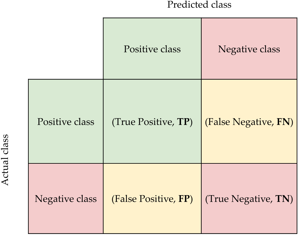
Figure S1. Confusion matrix.
From the confusion matrix, the measures employed in our experimental analysis are defined as follows:
- Accuracy: indicates the proportion of correct predictions irrespective of class. This measure is defined as:
(TP + TN) / (TP + TN + FP + FN) - Sensitivity: measures the proportion of positives that the classifier predicts correctly. This measure is defined as:
TP / (TP + FN) - Specificity: measures the proportion of negatives that the classifier predicts correctly. This measure is defined as:
TN / (TN + FP) - AUC: calculate the area under a ROC (Receiver Operator Characteristic) curve for a classifier. This measure is defined as:
(1 + Sensitivity - (1 - Specificity)) / 2 - G-mean: is the geometric mean between sensitivity and specificity, penalising the lower value. This measure is defined as:
√ Sensitivity * Specificity
All the presented classification measures take values in the range [0.0,1.0], representing a value of 1 in these measures the best predictive ability of the model and 0 the worst. In order to correctly evaluate the classifiers generated by a particular algorithm, the average of the measures together with their standard deviation must be studied in a statistically appropriate methodology known as k fold cross validation. Furthermore, it should be kept in mind that data limitations such as low sample size or high dimensionality can negatively affect the predictive quality of the classifier by showing lower values, on the other hand very high measure values are often an indicator of overfitting of the classifier and for this reason should be monitored [3].
Resampling methods
Other drawbacks to consider are class imbalance and low sample size, previously mentioned in the Section Introduction. The main issue of class imbalance is the learning process of ML algorithms that generate overfitted models toward the majority class examples. It results in that the minority examples are not well modelled and reflecting it in the classification measures by classes. To solve this limitation, we used different sampling methods (oversampling and undersampling) over the training folds to provide a balanced data distribution improving the learning process and the overall performance of classifiers [4]. Below, we described several resampling methods used in this work:
- SMOTE: a classical method inspired in k nearest neighbors that over-sampled by creating artificial examples belonging to the minority class.
- SMOTE-NC: a extension of the previous one that can handle categorical features.
- ADASYN: a improved version of the first one that randomly modifies the values slightly to make them more realistic.
- ROSE: this method generates new examples from the minority class estimating the conditional density of the two classes.
- NearMiss: this method uses the k nearest neighbors approach to select a subset of the majority class examples.
- TomeK: a technique that detects the Tomek's link between two examples of differentes classes and removed them.
Predictive methods analyzed
The classification algorithms used have been selected from a comparative study in which 179 classifiers from 17 families were evaluated. We chose algorithms from 5 different families such as the well-known interpretable decision trees, and the accurate Random Forest, Support Vector Machine and Neural Network. The algorithms chosen from the different families were:
- C4.5 [9]: This is a classical algorithm developed by Ross Quinlan that generates decision trees.
- Random Forest [6,8]: It is an algorithm that performs a random selection of variables to generate a large number of decision trees that are subsequently combined to carry out the prediction.
- xgBoost [1]: An algorithm generates a boosting type ensemble with the well-known gradient boosting cost function.
- svmRadialCost [5]: It is an algorithm that searches for the optimal hyperplane through a kernel function of the radial type, generating a model that usually discriminates classes quite successfully.
- avNNet [10]: It is an algorithm that creates a model based on a committee of several multi-layer perceptrons trained with different weight initializations.
Results
We used 5-fold cross validation with 5 repeats (25 executions in total) for each algorithm and resampling strategy during the training phase. We show the average results obtained (and standard deviation) for each quality measure on the test data sets when the models have been learned from the balanced training sets using each of the methods mentioned in the previous section. Note that, the table of results obtained using the NearMiss method is available in the paper since it is the resampling method that has allowed the different Machine Learning techniques to learn the best performing models on the test sets.
It should be noted that several classifiers were evaluated with the resampling methods explored in the different omics data layers (Gen; Genomic data, Epi; Epigenomic data and Clin; Clinical data). In addition, the predictive ability of the different combinations of omics data (Gen + Epi, Gen + Clin, Epi + Clin and All) was also evaluated under the same conditions.
Moreover, performance results are available for download in xls and csv files by clicking the icons ![]() and
and ![]() , respectively.
, respectively.
SMOTE
| Classification measures | ||||||
| Fusion | Methods | Accuracy | Sensitivity | Specificity | AUC | G_mean |
| Gen | RF | 0.72 (0.04) | 0.09 (0.10) | 0.98 (0.04) | 0.53 (0.05) | 0.21 (0.22) |
| xgBoost | 0.69 (0.10) | 0.29 (0.19) | 0.85 (0.11) | 0.57 (0.11) | 0.44 (0.23) | |
| C4.5 | 0.61 (0.09) | 0.33 (0.17) | 0.72 (0.13) | 0.53 (0.09) | 0.46 (0.15) | |
| svmRadial | 0.72 (0.10) | 0.28 (0.21) | 0.90 (0.11) | 0.59 (0.12) | 0.44 (0.26) | |
| avNNet | 0.71 (0.07) | 0.42 (0.21) | 0.83 (0.09) | 0.62 (0.10) | 0.56 (0.17) | |
| Fusion | Methods | Accuracy | Sensitivity | Specificity | AUC | G_mean |
| Epi | RF | 0.70 (0.08) | 0.18 (0.17) | 0.90 (0.10) | 0.54 (0.09) | 0.31 (0.25) |
| xgBoost | 0.75 (0.09) | 0.51 (0.24) | 0.84 (0.10) | 0.67 (0.12) | 0.62 (0.20) | |
| C4.5 | 0.63 (0.10) | 0.38 (0.21) | 0.73 (0.12) | 0.55 (0.12) | 0.47 (0.23) | |
| svmRadial | 0.71 (0.10) | 0.33 (0.23) | 0.87 (0.12) | 0.60 (0.12) | 0.48 (0.25) | |
| avNNet | 0.39 (0.20) | 0.86 (0.32) | 0.20 (0.38) | 0.53 (0.11) | 0.11 (0.26) | |
| Fusion | Methods | Accuracy | Sensitivity | Specificity | AUC | G_mean |
| Clin | RF | 0.66 (0.10) | 0.44 (0.26) | 0.75 (0.12) | 0.59 (0.14) | 0.53 (0.21) |
| xgBoost | 0.61 (0.10) | 0.36 (0.19) | 0.71 (0.13) | 0.53 (0.11) | 0.46 (0.20) | |
| C4.5 | 0.61 (0.09) | 0.42 (0.21) | 0.69 (0.10) | 0.56 (0.12) | 0.51 (0.19) | |
| svmRadial | 0.65 (0.12) | 0.47 (0.21) | 0.72 (0.17) | 0.59 (0.12) | 0.56 (0.13) | |
| avNNet | 0.69 (0.05) | 0.02 (0.09) | 0.96 (0.10) | 0.49 (0.03) | 0.04 (0.12) | |
| Fusion | Methods | Accuracy | Sensitivity | Specificity | AUC | G_mean |
| Gen + Epi | RF | 0.72 (0.05) | 0.13 (0.14) | 0.95 (0.05) | 0.54 (0.07) | 0.25 (0.25) |
| xgBoost | 0.71 (0.09) | 0.37 (0.23) | 0.85 (0.10) | 0.61 (0.12) | 0.52 (0.22) | |
| C4.5 | 0.63 (0.08) | 0.35 (0.21) | 0.74 (0.12) | 0.55 (0.10) | 0.45 (0.22) | |
| svmRadial | 0.71 (0.09) | 0.31 (0.20) | 0.87 (0.11) | 0.59 (0.10) | 0.46 (0.23) | |
| avNNet | 0.59 (0.20) | 0.55 (0.36) | 0.61 (0.39) | 0.58 (0.11) | 0.37 (0.30) | |
| Fusion | Methods | Accuracy | Sensitivity | Specificity | AUC | G_mean |
| Gen + Clin | RF | 0.72 (0.07) | 0.23 (0.18) | 0.91 (0.08) | 0.57 (0.09) | 0.39 (0.25) |
| xgBoost | 0.64 (0.10) | 0.31 (0.19) | 0.77 (0.12) | 0.54 (0.11) | 0.46 (0.17) | |
| C4.5 | 0.65 (0.09) | 0.35 (0.25) | 0.77 (0.11) | 0.56 (0.12) | 0.45 (0.25) | |
| svmRadial | 0.71 (0.09) | 0.42 (0.28) | 0.83 (0.11) | 0.62 (0.13) | 0.53 (0.25) | |
| avNNet | 0.50 (0.16) | 0.47 (0.31) | 0.50 (0.28) | 0.49 (0.12) | 0.35 (0.24) | |
| Fusion | Methods | Accuracy | Sensitivity | Specificity | AUC | G_mean |
| Epi + Clin | RF | 0.73 (0.06) | 0.29 (0.20) | 0.91 (0.08) | 0.60 (0.09) | 0.45 (0.23) |
| xgBoost | 0.69 (0.08) | 0.41 (0.19) | 0.81 (0.09) | 0.61 (0.10) | 0.55 (0.16) | |
| C4.5 | 0.65 (0.08) | 0.39 (0.25) | 0.76 (0.10) | 0.57 (0.12) | 0.49 (0.22) | |
| svmRadial | 0.73 (0.07) | 0.38 (0.26) | 0.87 (0.11) | 0.63 (0.10) | 0.51 (0.24) | |
| avNNet | 0.46 (0.16) | 0.61 (0.33) | 0.40 (0.31) | 0.51 (0.11) | 0.37 (0.20) | |
| Fusion | Methods | Accuracy | Sensitivity | Specificity | AUC | G_mean |
| All | RF | 0.74 (0.05) | 0.19 (0.17) | 0.96 (0.05) | 0.57 (0.08) | 0.34 (0.27) |
| xgBoost | 0.69 (0.08) | 0.36 (0.17) | 0.82 (0.09) | 0.59 (0.09) | 0.51 (0.18) | |
| C4.5 | 0.65 (0.10) | 0.38 (0.22) | 0.75 (0.12) | 0.57 (0.11) | 0.49 (0.21) | |
| svmRadial | 0.72 (0.08) | 0.31 (0.24) | 0.89 (0.08) | 0.60 (0.12) | 0.45 (0.27) | |
| avNNet | 0.51 (0.12) | 0.51 (0.33) | 0.51 (0.22) | 0.51 (0.13) | 0.40 (0.23) | |
Table S3. Average and standard deviations results for each algorithm in the training stage (5-fold cross validation with 5 repeats) for each layer or data fusion using the oversampling method SMOTE. ![]()
![]()
SMOTE_NC
| Classification measures | ||||||
| Fusion | Methods | Accuracy | Sensitivity | Specificity | AUC | G_mean |
| Gen | RF | 0.72 (0.03) | 0.08 (0.11) | 0.98 (0.03) | 0.53 (0.05) | 0.18 (0.22) |
| xgBoost | 0.66 (0.07) | 0.23 (0.13) | 0.83 (0.10) | 0.53 (0.07) | 0.39 (0.19) | |
| C4.5 | 0.59 (0.10) | 0.31 (0.18) | 0.71 (0.12) | 0.51 (0.10) | 0.43 (0.17) | |
| svmRadial | 0.71 (0.08) | 0.30 (0.23) | 0.88 (0.11) | 0.59 (0.11) | 0.43 (0.27) | |
| avNNet | 0.69 (0.06) | 0.37 (0.24) | 0.82 (0.09) | 0.60 (0.10) | 0.49 (0.23) | |
| Fusion | Methods | Accuracy | Sensitivity | Specificity | AUC | G_mean |
| Epi | RF | 0.70 (0.06) | 0.20 (0.15) | 0.91 (0.08) | 0.56 (0.07) | 0.36 (0.22) |
| xgBoost | 0.71 (0.10) | 0.43 (0.23) | 0.82 (0.11) | 0.62 (0.13) | 0.56 (0.19) | |
| C4.5 | 0.60 (0.12) | 0.37 (0.20) | 0.70 (0.15) | 0.54 (0.12) | 0.48 (0.18) | |
| svmRadial | 0.70 (0.11) | 0.38 (0.26) | 0.83 (0.12) | 0.60 (0.14) | 0.49 (0.26) | |
| avNNet | 0.38 (0.18) | 0.90 (0.25) | 0.16 (0.34) | 0.53 (0.08) | 0.11 (0.25) | |
| Fusion | Methods | Accuracy | Sensitivity | Specificity | AUC | G_mean |
| Clin | RF | 0.66 (0.09) | 0.35 (0.20) | 0.78 (0.12) | 0.57 (0.11) | 0.49 (0.19) |
| xgBoost | 0.60 (0.10) | 0.36 (0.23) | 0.70 (0.12) | 0.53 (0.12) | 0.43 (0.24) | |
| C4.5 | 0.61 (0.09) | 0.37 (0.25) | 0.71 (0.08) | 0.54 (0.13) | 0.47 (0.22) | |
| svmRadial | 0.64 (0.12) | 0.47 (0.19) | 0.71 (0.16) | 0.59 (0.12) | 0.56 (0.13) | |
| avNNet | 0.68 (0.09) | 0.06 (0.21) | 0.93 (0.21) | 0.50 (0.02) | 0.04 (0.13) | |
| Fusion | Methods | Accuracy | Sensitivity | Specificity | AUC | G_mean |
| Gen + Epi | RF | 0.72 (0.05) | 0.11 (0.13) | 0.96 (0.06) | 0.54 (0.07) | 0.22 (0.24) |
| xgBoost | 0.70 (0.08) | 0.37 (0.23) | 0.84 (0.10) | 0.60 (0.11) | 0.51 (0.21) | |
| C4.5 | 0.61 (0.08) | 0.37 (0.18) | 0.71 (0.11) | 0.54 (0.08) | 0.48 (0.14) | |
| svmRadial | 0.69 (0.12) | 0.34 (0.25) | 0.83 (0.14) | 0.58 (0.14) | 0.47 (0.25) | |
| avNNet | 0.58 (0.21) | 0.56 (0.29) | 0.59 (0.37) | 0.58 (0.11) | 0.42 (0.27) | |
| Fusion | Methods | Accuracy | Sensitivity | Specificity | AUC | G_mean |
| Gen + Clin | RF | 0.69 (0.07) | 0.17 (0.16) | 0.91 (0.08) | 0.54 (0.08) | 0.32 (0.23) |
| xgBoost | 0.66 (0.09) | 0.35 (0.25) | 0.78 (0.13) | 0.57 (0.12) | 0.45 (0.26) | |
| C4.5 | 0.66 (0.09) | 0.42 (0.28) | 0.77 (0.12) | 0.59 (0.12) | 0.50 (0.25) | |
| svmRadial | 0.74 (0.07) | 0.42 (0.27) | 0.87 (0.09) | 0.65 (0.12) | 0.55 (0.23) | |
| avNNet | 0.52 (0.17) | 0.54 (0.34) | 0.51 (0.34) | 0.53 (0.11) | 0.36 (0.26) | |
| Fusion | Methods | Accuracy | Sensitivity | Specificity | AUC | G_mean |
| Epi + Clin | RF | 0.74 (0.07) | 0.28 (0.22) | 0.92 (0.08) | 0.60 (0.10) | 0.44 (0.25) |
| xgBoost | 0.70 (0.09) | 0.39 (0.19) | 0.82 (0.11) | 0.60 (0.10) | 0.54 (0.14) | |
| C4.5 | 0.67 (0.08) | 0.41 (0.21) | 0.77 (0.09) | 0.59 (0.11) | 0.53 (0.19) | |
| svmRadial | 0.76 (0.08) | 0.37 (0.27) | 0.92 (0.10) | 0.64 (0.12) | 0.50 (0.27) | |
| avNNet | 0.46 (0.14) | 0.62 (0.29) | 0.39 (0.27) | 0.50 (0.10) | 0.39 (0.19) | |
| Fusion | Methods | Accuracy | Sensitivity | Specificity | AUC | G_mean |
| All | RF | 0.73 (0.06) | 0.20 (0.16) | 0.95 (0.07) | 0.58 (0.08) | 0.35 (0.26) |
| xgBoost | 0.70 (0.07) | 0.36 (0.16) | 0.84 (0.09) | 0.60 (0.08) | 0.53 (0.15) | |
| C4.5 | 0.64 (0.11) | 0.37 (0.18) | 0.75 (0.13) | 0.56 (0.11) | 0.51 (0.16) | |
| svmRadial | 0.72 (0.08) | 0.33 (0.22) | 0.88 (0.10) | 0.60 (0.10) | 0.47 (0.24) | |
| avNNet | 0.50 (0.14) | 0.46 (0.28) | 0.52 (0.22) | 0.49 (0.13) | 0.40 (0.22) | |
Table S4. Average and standard deviations results for each algorithm in the training stage (5-fold cross validation with 5 repeats) for each layer or data fusion using the oversampling method SMOTE_NC. ![]()
![]()
ADASYN
| Classification measures | ||||||
| Fusion | Methods | Accuracy | Sensitivity | Specificity | AUC | G_mean |
| Gen | RF | 0.72 (0.04) | 0.09 (0.11) | 0.98 (0.04) | 0.53 (0.06) | 0.18 (0.23) |
| xgBoost | 0.66 (0.08) | 0.26 (0.16) | 0.83 (0.09) | 0.54 (0.09) | 0.42 (0.21) | |
| C4.5 | 0.59 (0.07) | 0.28 (0.22) | 0.71 (0.10) | 0.50 (0.10) | 0.38 (0.22) | |
| svmRadial | 0.68 (0.09) | 0.28 (0.20) | 0.84 (0.10) | 0.56 (0.11) | 0.43 (0.24) | |
| avNNet | 0.65 (0.07) | 0.41 (0.20) | 0.74 (0.11) | 0.58 (0.09) | 0.51 (0.18) | |
| Fusion | Methods | Accuracy | Sensitivity | Specificity | AUC | G_mean |
| Epi | RF | 0.71 (0.07) | 0.18 (0.12) | 0.92 (0.09) | 0.55 (0.07) | 0.36 (0.20) |
| xgBoost | 0.72 (0.10) | 0.47 (0.19) | 0.82 (0.13) | 0.65 (0.10) | 0.60 (0.18) | |
| C4.5 | 0.63 (0.13) | 0.40 (0.19) | 0.73 (0.15) | 0.56 (0.13) | 0.51 (0.17) | |
| svmRadial | 0.72 (0.10) | 0.39 (0.26) | 0.85 (0.13) | 0.62 (0.13) | 0.52 (0.24) | |
| avNNet | 0.40 (0.19) | 0.82 (0.32) | 0.23 (0.38) | 0.53 (0.07) | 0.13 (0.26) | |
| Fusion | Methods | Accuracy | Sensitivity | Specificity | AUC | G_mean |
| Clin | RF | 0.63 (0.09) | 0.37 (0.15) | 0.74 (0.11) | 0.55 (0.10) | 0.50 (0.14) |
| xgBoost | 0.59 (0.10) | 0.30 (0.20) | 0.71 (0.13) | 0.50 (0.11) | 0.41 (0.21) | |
| C4.5 | 0.60 (0.10) | 0.39 (0.24) | 0.68 (0.11) | 0.54 (0.13) | 0.47 (0.22) | |
| svmRadial | 0.63 (0.12) | 0.49 (0.14) | 0.69 (0.19) | 0.59 (0.10) | 0.57 (0.10) | |
| avNNet | 0.68 (0.10) | 0.05 (0.20) | 0.93 (0.21) | 0.49 (0.05) | 0.03 (0.12) | |
| Fusion | Methods | Accuracy | Sensitivity | Specificity | AUC | G_mean |
| Gen + Epi | RF | 0.72 (0.05) | 0.10 (0.14) | 0.97 (0.05) | 0.53 (0.08) | 0.20 (0.24) |
| xgBoost | 0.71 (0.10) | 0.40 (0.20) | 0.84 (0.10) | 0.62 (0.12) | 0.55 (0.18) | |
| C4.5 | 0.59 (0.10) | 0.37 (0.20) | 0.68 (0.14) | 0.53 (0.11) | 0.47 (0.18) | |
| svmRadial | 0.69 (0.09) | 0.33 (0.18) | 0.83 (0.12) | 0.58 (0.09) | 0.49 (0.19) | |
| avNNet | 0.56 (0.20) | 0.55 (0.38) | 0.56 (0.38) | 0.56 (0.12) | 0.32 (0.32) | |
| Fusion | Methods | Accuracy | Sensitivity | Specificity | AUC | G_mean |
| Gen + Clin | RF | 0.72 (0.07) | 0.20 (0.20) | 0.92 (0.07) | 0.56 (0.10) | 0.34 (0.28) |
| xgBoost | 0.67 (0.11) | 0.36 (0.23) | 0.80 (0.15) | 0.58 (0.12) | 0.50 (0.18) | |
| C4.5 | 0.67 (0.12) | 0.41 (0.30) | 0.77 (0.12) | 0.59 (0.16) | 0.49 (0.29) | |
| svmRadial | 0.72 (0.10) | 0.38 (0.26) | 0.87 (0.11) | 0.62 (0.13) | 0.51 (0.26) | |
| avNNet | 0.56 (0.15) | 0.42 (0.35) | 0.61 (0.31) | 0.51 (0.09) | 0.33 (0.24) | |
| Fusion | Methods | Accuracy | Sensitivity | Specificity | AUC | G_mean |
| Epi + Clin | RF | 0.74 (0.05) | 0.28 (0.19) | 0.92 (0.07) | 0.60 (0.09) | 0.45 (0.23) |
| xgBoost | 0.69 (0.09) | 0.39 (0.18) | 0.82 (0.12) | 0.60 (0.09) | 0.54 (0.16) | |
| C4.5 | 0.66 (0.12) | 0.46 (0.24) | 0.74 (0.12) | 0.60 (0.15) | 0.55 (0.21) | |
| svmRadial | 0.72 (0.05) | 0.37 (0.27) | 0.87 (0.10) | 0.62 (0.10) | 0.49 (0.25) | |
| avNNet | 0.43 (0.14) | 0.66 (0.29) | 0.34 (0.23) | 0.50 (0.14) | 0.40 (0.20) | |
| Fusion | Methods | Accuracy | Sensitivity | Specificity | AUC | G_mean |
| All | RF | 0.73 (0.05) | 0.19 (0.15) | 0.95 (0.06) | 0.57 (0.07) | 0.35 (0.24) |
| xgBoost | 0.70 (0.08) | 0.42 (0.20) | 0.82 (0.11) | 0.62 (0.10) | 0.55 (0.19) | |
| C4.5 | 0.64 (0.11) | 0.38 (0.21) | 0.74 (0.14) | 0.56 (0.12) | 0.50 (0.18) | |
| svmRadial | 0.73 (0.06) | 0.34 (0.21) | 0.88 (0.09) | 0.61 (0.09) | 0.49 (0.22) | |
| avNNet | 0.48 (0.13) | 0.46 (0.33) | 0.49 (0.22) | 0.48 (0.13) | 0.36 (0.23) | |
Table S5. Average and standard deviations results for each algorithm in the training stage (5-fold cross validation with 5 repeats) for each layer or data fusion using the oversampling method ADASYN. ![]()
![]()
ROSE
| Classification measures | ||||||
| Fusion | Methods | Accuracy | Sensitivity | Specificity | AUC | G_mean |
| Gen | RF | 0.33 (0.09) | 0.86 (0.15) | 0.12 (0.13) | 0.49 (0.09) | 0.24 (0.19) |
| xgBoost | 0.32 (0.06) | 0.93 (0.13) | 0.07 (0.06) | 0.50 (0.07) | 0.20 (0.15) | |
| C4.5 | 0.31 (0.07) | 0.91 (0.16) | 0.07 (0.05) | 0.49 (0.09) | 0.21 (0.14) | |
| svmRadial | 0.57 (0.16) | 0.59 (0.21) | 0.57 (0.22) | 0.58 (0.14) | 0.54 (0.18) | |
| avNNet | 0.56 (0.12) | 0.63 (0.19) | 0.53 (0.15) | 0.58 (0.12) | 0.56 (0.12) | |
| Fusion | Methods | Accuracy | Sensitivity | Specificity | AUC | G_mean |
| Epi | RF | 0.42 (0.12) | 0.93 (0.11) | 0.21 (0.16) | 0.57 (0.11) | 0.40 (0.20) |
| xgBoost | 0.47 (0.10) | 0.77 (0.19) | 0.35 (0.14) | 0.56 (0.10) | 0.49 (0.12) | |
| C4.5 | 0.45 (0.09) | 0.76 (0.20) | 0.32 (0.13) | 0.54 (0.10) | 0.47 (0.14) | |
| svmRadial | 0.59 (0.14) | 0.69 (0.23) | 0.55 (0.18) | 0.62 (0.14) | 0.59 (0.15) | |
| avNNet | 0.30 (0.03) | 0.99 (0.04) | 0.01 (0.06) | 0.50 (0.01) | 0.02 (0.10) | |
| Fusion | Methods | Accuracy | Sensitivity | Specificity | AUC | G_mean |
| Clin | RF | 0.48 (0.11) | 0.79 (0.18) | 0.36 (0.15) | 0.57 (0.11) | 0.51 (0.12) |
| xgBoost | 0.51 (0.14) | 0.58 (0.20) | 0.49 (0.19) | 0.54 (0.12) | 0.50 (0.16) | |
| C4.5 | 0.45 (0.13) | 0.62 (0.24) | 0.38 (0.17) | 0.50 (0.13) | 0.46 (0.14) | |
| svmRadial | 0.53 (0.13) | 0.64 (0.20) | 0.49 (0.15) | 0.56 (0.14) | 0.55 (0.15) | |
| avNNet | 0.30 (0.06) | 0.92 (0.17) | 0.05 (0.12) | 0.48 (0.05) | 0.07 (0.15) | |
| Fusion | Methods | Accuracy | Sensitivity | Specificity | AUC | G_mean |
| Gen + Epi | RF | 0.35 (0.10) | 0.91 (0.16) | 0.12 (0.10) | 0.52 (0.11) | 0.29 (0.18) |
| xgBoost | 0.30 (0.07) | 0.90 (0.18) | 0.06 (0.08) | 0.48 (0.09) | 0.17 (0.16) | |
| C4.5 | 0.31 (0.07) | 0.90 (0.18) | 0.07 (0.09) | 0.48 (0.09) | 0.17 (0.16) | |
| svmRadial | 0.60 (0.11) | 0.56 (0.25) | 0.62 (0.16) | 0.59 (0.12) | 0.55 (0.17) | |
| avNNet | 0.46 (0.18) | 0.74 (0.28) | 0.35 (0.32) | 0.54 (0.10) | 0.32 (0.30) | |
| Fusion | Methods | Accuracy | Sensitivity | Specificity | AUC | G_mean |
| Gen + Clin | RF | 0.33 (0.09) | 0.86 (0.18) | 0.11 (0.10) | 0.48 (0.11) | 0.25 (0.18) |
| xgBoost | 0.30 (0.07) | 0.90 (0.18) | 0.06 (0.08) | 0.48 (0.09) | 0.17 (0.16) | |
| C4.5 | 0.31 (0.07) | 0.90 (0.18) | 0.07 (0.09) | 0.48 (0.09) | 0.17 (0.16) | |
| svmRadial | 0.59 (0.12) | 0.45 (0.27) | 0.65 (0.16) | 0.55 (0.13) | 0.48 (0.22) | |
| avNNet | 0.28 (0.02) | 0.96 (0.09) | 0.01 (0.03) | 0.49 (0.03) | 0.02 (0.08) | |
| Fusion | Methods | Accuracy | Sensitivity | Specificity | AUC | G_mean |
| Epi + Clin | RF | 0.44 (0.09) | 0.89 (0.16) | 0.25 (0.12) | 0.57 (0.09) | 0.45 (0.12) |
| xgBoost | 0.49 (0.14) | 0.79 (0.19) | 0.37 (0.18) | 0.58 (0.12) | 0.52 (0.14) | |
| C4.5 | 0.46 (0.13) | 0.75 (0.20) | 0.34 (0.17) | 0.54 (0.12) | 0.48 (0.14) | |
| svmRadial | 0.61 (0.12) | 0.67 (0.19) | 0.58 (0.14) | 0.62 (0.13) | 0.61 (0.13) | |
| avNNet | 0.28 (0.02) | 0.96 (0.16) | 0.01 (0.05) | 0.48 (0.06) | 0.01 (0.04) | |
| Fusion | Methods | Accuracy | Sensitivity | Specificity | AUC | G_mean |
| All | RF | 0.37 (0.10) | 0.91 (0.16) | 0.15 (0.10) | 0.53 (0.11) | 0.34 (0.17) |
| xgBoost | 0.30 (0.07) | 0.90 (0.18) | 0.06 (0.08) | 0.48 (0.09) | 0.16 (0.16) | |
| C4.5 | 0.31 (0.07) | 0.90 (0.18) | 0.07 (0.09) | 0.48 (0.09) | 0.17 (0.16) | |
| svmRadial | 0.61 (0.14) | 0.64 (0.21) | 0.60 (0.18) | 0.62 (0.13) | 0.60 (0.14) | |
| avNNet | 0.30 (0.05) | 0.97 (0.07) | 0.03 (0.08) | 0.50 (0.03) | 0.07 (0.15) | |
Table S6. Average and standard deviations results for each algorithm in the training stage (5-fold cross validation with 5 repeats) for each layer or data fusion using the oversampling method ROSE. ![]()
![]()
Tomek
| Classification measures | ||||||
| Fusion | Methods | Accuracy | Sensitivity | Specificity | AUC | G_mean |
| Gen | RF | 0.72 (0.02) | 0.02 (0.06) | 1 (0) | 0.51 (0.03) | 0.05 (0.14) |
| xgBoost | 0.68 (0.08) | 0.21 (0.17) | 0.87 (0.10) | 0.54 (0.09) | 0.35 (0.24) | |
| C4.5 | 0.58 (0.10) | 0.20 (0.16) | 0.74 (0.13) | 0.47 (0.09) | 0.32 (0.21) | |
| svmRadial | 0.75 (0.05) | 0.14 (0.14) | 0.99 (0.02) | 0.57 (0.07) | 0.27 (0.26) | |
| avNNet | 0.73 (0.07) | 0.24 (0.18) | 0.92 (0.09) | 0.58 (0.08) | 0.40 (0.23) | |
| Fusion | Methods | Accuracy | Sensitivity | Specificity | AUC | G_mean |
| Epi | RF | 0.71 (0.03) | 0.01 (0.04) | 0.99 (0.03) | 0.50 (0.02) | 0.02 (0.09) |
| xgBoost | 0.70 (0.07) | 0.18 (0.17) | 0.91 (0.09) | 0.55 (0.09) | 0.32 (0.26) | |
| C4.5 | 0.63 (0.10) | 0.28 (0.17) | 0.78 (0.14) | 0.53 (0.10) | 0.43 (0.17) | |
| svmRadial | 0.77 (0.10) | 0.39 (0.23) | 0.92 (0.09) | 0.66 (0.14) | 0.55 (0.25) | |
| avNNet | 0.71 (0.02) | 0 (0) | 1 (0) | 0.50 (0) | 0 (0) | |
| Fusion | Methods | Accuracy | Sensitivity | Specificity | AUC | G_mean |
| Clin | RF | 0.68 (0.06) | 0.05 (0.10) | 0.94 (0.08) | 0.49 (0.06) | 0.09 (0.19) |
| xgBoost | 0.65 (0.09) | 0.21 (0.16) | 0.83 (0.10) | 0.52 (0.10) | 0.37 (0.21) | |
| C4.5 | 0.62 (0.08) | 0.28 (0.23) | 0.76 (0.10) | 0.52 (0.11) | 0.40 (0.22) | |
| svmRadial | 0.68 (0.08) | 0.01 (0.04) | 0.96 (0.10) | 0.48 (0.06) | 0.02 (0.09) | |
| avNNet | 0.71 (0.02) | 0 (0) | 1 (0) | 0.50 (0) | 0 (0) | |
| Fusion | Methods | Accuracy | Sensitivity | Specificity | AUC | G_mean |
| Gen + Epi | RF | 0.71 (0.02) | 0 (0) | 1 (0.02) | 0.50 (0.01) | 0 (0) |
| xgBoost | 0.70 (0.08) | 0.21 (0.19) | 0.90 (0.09) | 0.55 (0.10) | 0.33 (0.27) | |
| C4.5 | 0.60 (0.11) | 0.23 (0.19) | 0.75 (0.12) | 0.49 (0.12) | 0.35 (0.24) | |
| svmRadial | 0.72 (0.08) | 0.18 (0.17) | 0.94 (0.12) | 0.56 (0.09) | 0.32 (0.26) | |
| avNNet | 0.71 (0.02) | 0 (0) | 1 (0) | 0.50 (0) | 0 (0) | |
| Fusion | Methods | Accuracy | Sensitivity | Specificity | AUC | G_mean |
| Gen + Clin | RF | 0.71 (0.03) | 0.04 (0.08) | 0.98 (0.04) | 0.51 (0.04) | 0.09 (0.18) |
| xgBoost | 0.69 (0.06) | 0.21 (0.19) | 0.88 (0.09) | 0.55 (0.08) | 0.34 (0.25) | |
| C4.5 | 0.64 (0.07) | 0.24 (0.20) | 0.80 (0.11) | 0.52 (0.09) | 0.35 (0.24) | |
| svmRadial | 0.70 (0.08) | 0.07 (0.12) | 0.95 (0.12) | 0.51 (0.07) | 0.14 (0.22) | |
| avNNet | 0.71 (0.02) | 0 (0) | 1 (0) | 0.50 (0) | 0 (0) | |
| Fusion | Methods | Accuracy | Sensitivity | Specificity | AUC | G_mean |
| Epi + Clin | RF | 0.70 (0.02) | 0 (0) | 0.99 (0.03) | 0.49 (0.01) | 0 (0) |
| xgBoost | 0.68 (0.07) | 0.14 (0.11) | 0.89 (0.10) | 0.52 (0.07) | 0.29 (0.21) | |
| C4.5 | 0.63 (0.10) | 0.33 (0.23) | 0.75 (0.12) | 0.54 (0.12) | 0.44 (0.23) | |
| svmRadial | 0.74 (0.07) | 0.30 (0.22) | 0.93 (0.08) | 0.61 (0.10) | 0.45 (0.26) | |
| avNNet | 0.71 (0.02) | 0 (0) | 1 (0) | 0.50 (0) | 0 (0) | |
| Fusion | Methods | Accuracy | Sensitivity | Specificity | AUC | G_mean |
| All | RF | 0.70 (0.03) | 0.01 (0.04) | 0.99 (0.03) | 0.50 (0.03) | 0.02 (0.09) |
| xgBoost | 0.69 (0.06) | 0.16 (0.12) | 0.90 (0.09) | 0.53 (0.06) | 0.32 (0.21) | |
| C4.5 | 0.65 (0.09) | 0.37 (0.23) | 0.76 (0.10) | 0.57 (0.11) | 0.48 (0.22) | |
| svmRadial | 0.70 (0.07) | 0.15 (0.17) | 0.92 (0.12) | 0.53 (0.08) | 0.25 (0.26) | |
| avNNet | 0.71 (0.02) | 0 (0) | 1 (0) | 0.50 (0) | 0 (0) | |
Table S7. Average and standard deviations results for each algorithm in the training stage (5-fold cross validation with 5 repeats) for each layer or data fusion using the oversampling method Tomek. ![]()
![]()
Explainability
Understanding the hidden reason why a black box model makes a prediction is vital in many applications. However, interpreting these complex classifiers has been the bottleneck for many years, making practitioners opt for simpler models in search of that understanding. In response, innovative methodologies have been developed, such as SHAP, which assigns each variable a value of importance for the prediction of each specific example [2].
Table S8 shows the top features sorted according to their importance in our final classifier (RF generated with all the dataset using NearMiss method), showing the mean, mininum, maximum, median, quantiles 1 and 3 contributions of each feature, ranked according to their importance. This table is available for download in xls and csv files by clicking the icons ![]() and
and ![]() , respectively.
, respectively.
| SHAP values | ||||||
| Feature | Min | Q1 | Median | Mean | Q3 | Max |
| cg11762807_HDAC4 | -0.0383836 | -0.0188528 | 0.0109172 | -0.0000344 | 0.0182584 | 0.0224375 |
| cg04976245_PTPRN2 | -0.0220381 | -0.0133175 | 0.0058597 | -0.0000203 | 0.0111599 | 0.0151985 |
| cg27147114_RASGRF1 | -0.0194180 | -0.0078942 | 0.0034873 | 0.0000426 | 0.0101327 | 0.0130818 |
| cg07792979_MATN2 | -0.0180166 | -0.0113417 | 0.0044036 | 0.0000043 | 0.0085169 | 0.0137533 |
| cg03516256_EBF1 | -0.0114256 | -0.0086135 | -0.0040286 | 0.0000015 | 0.0095440 | 0.0137712 |
| Leptin_adiponectin_ratio | -0.0234292 | -0.0094655 | 0.0050250 | -0.0000530 | 0.0080091 | 0.0096243 |
| cg16486501_PTPRN2 | -0.0120017 | -0.0078438 | 0.0023604 | 0.0000191 | 0.0071751 | 0.0117088 |
| cg19194924 | -0.0087772 | -0.0071610 | -0.0040971 | 0.0000387 | 0.0104498 | 0.0159478 |
| BMI_zscore | -0.0186424 | -0.0050623 | 0.0037218 | 0.0000396 | 0.0070041 | 0.0095406 |
| Iron_(ug/dl) | -0.0070307 | -0.0061667 | -0.0029898 | 0.0000729 | 0.0075218 | 0.0147095 |
| cg02818143_PTPRN2 | -0.0146732 | -0.0056237 | -0.0004137 | -0.0000404 | 0.0069536 | 0.0123840 |
| Leptin_(ug/l) | -0.0179066 | -0.0036802 | 0.0033796 | -0.0000486 | 0.0059580 | 0.0080283 |
| cg14299905_MAP4 | -0.0069842 | -0.0055708 | -0.0034039 | 0.0000342 | 0.0075290 | 0.0135848 |
| cg10937973_CLASP1 | -0.0103603 | -0.0045720 | -0.0003926 | 0.0000375 | 0.0055592 | 0.0075534 |
| HDLc_(mg/dl) | -0.0069388 | -0.0046289 | -0.0018813 | -0.0000338 | 0.0042094 | 0.0110115 |
| cg13687935_MYT1L | -0.0109815 | -0.0054153 | 0.0000000 | -0.0000583 | 0.0038894 | 0.0086981 |
| cg21549415_P4HB | -0.0078892 | -0.0051169 | 0.0000000 | 0.0000214 | 0.0027630 | 0.0111581 |
| cg10987850_HMCN1 | -0.0160627 | -0.0090381 | 0.0015998 | -0.0000447 | 0.0034693 | 0.0181333 |
| cg23792592_MIR1-1 | -0.0081381 | -0.0048317 | 0.0020805 | 0.0000072 | 0.0039073 | 0.0071372 |
| cg00152126_CTBP2 | -0.0126719 | -0.0036879 | 0.0024147 | 0.0000400 | 0.0042828 | 0.0060726 |
| cg16892627_MTHFD1L | -0.0094311 | -0.0030475 | 0.0009467 | -0.0000316 | 0.0038131 | 0.0068254 |
| cg16306644_COX19 | -0.0090327 | -0.0032348 | 0.0000000 | -0.0000402 | 0.0040988 | 0.0087172 |
| cg15168723_BRD1 | -0.0071609 | -0.0035901 | -0.0018249 | 0.0000442 | 0.0042765 | 0.0089177 |
| Blood_proteins_(g/dl) | -0.0063810 | -0.0039973 | -0.0026415 | 0.0000155 | 0.0002278 | 0.0177570 |
| cg12913090_ATG2B | -0.0110450 | -0.0018779 | 0.0024910 | -0.0000281 | 0.0037767 | 0.0054184 |
| cg02283975_STK36 | -0.0082249 | -0.0037287 | 0.0017228 | 0.0000433 | 0.0034778 | 0.0052090 |
| cg22151387_GRID1 | -0.0101193 | -0.0036806 | 0.0018482 | -0.0000090 | 0.0032653 | 0.0052139 |
| cg18073874_EEFSEC | -0.0128491 | -0.0013090 | 0.0019578 | -0.0000273 | 0.0037237 | 0.0055908 |
| cg12700273_RAPGEF4 | -0.0068050 | -0.0035348 | 0.0011904 | -0.0000557 | 0.0027735 | 0.0046711 |
| cg26624881_CLPTM1L | -0.0052119 | -0.0029128 | 0.0000000 | -0.0000364 | 0.0033781 | 0.0045530 |
Table S8. Summary of feature contributions to the final classifier for IR and non-IR samples. Mean, mininum, maximum, median, quantiles 1 and 3 are shown for each sample group. ![]()
![]()
Table S8 can be divided into two further tables showing the contribution of variables in examples predicted as IR or non-IR, which are shown below (Table S9 and Table S10).
| IR children (positive class) SHAP values | ||||||
| Feature | Min | Q1 | Median | Mean | Q3 | Max |
| cg11762807_HDAC4 | -0.0188115 | 0.0165476 | 0.0182611 | 0.0142781 | 0.0189999 | 0.0224375 |
| cg04976245_PTPRN2 | -0.0120716 | 0.0079529 | 0.0112535 | 0.0081016 | 0.0133654 | 0.0151985 |
| cg27147114_RASGRF1 | -0.0121908 | 0.0042595 | 0.0101629 | 0.0071670 | 0.0112826 | 0.0130818 |
| cg07792979_MATN2 | -0.0107621 | 0.0063719 | 0.0085562 | 0.0062697 | 0.0101399 | 0.0137533 |
| cg03516256_EBF1 | -0.0067574 | -0.0040903 | 0.0095992 | 0.0055053 | 0.0112740 | 0.0137712 |
| Leptin_adiponectin_ratio | -0.0117891 | 0.0072796 | 0.0080141 | 0.0064348 | 0.0081895 | 0.0096243 |
| cg16486501_PTPRN2 | -0.0073085 | 0.0020884 | 0.0072084 | 0.0046759 | 0.0086099 | 0.0117088 |
| cg19194924 | -0.0050127 | -0.0035934 | 0.0104603 | 0.0052300 | 0.0115948 | 0.0159478 |
| BMI_zscore | -0.0050450 | 0.0050537 | 0.0070662 | 0.0053662 | 0.0080135 | 0.0095406 |
| Iron_(ug/dl) | -0.0050651 | -0.0027281 | 0.0037389 | 0.0045182 | 0.0120790 | 0.0147095 |
| cg02818143_PTPRN2 | -0.0052860 | -0.0013407 | 0.0064526 | 0.0048223 | 0.0096586 | 0.0123840 |
| Leptin_(ug/l) | -0.0067801 | 0.0043171 | 0.0059613 | 0.0047006 | 0.0065667 | 0.0080283 |
| cg14299905_MAP4 | -0.0043411 | -0.0029141 | 0.0013899 | 0.0036786 | 0.0109645 | 0.0135848 |
| cg10937973_CLASP1 | -0.0062389 | -0.0007581 | 0.0055336 | 0.0031173 | 0.0065030 | 0.0075534 |
| HDLc_(mg/dl) | -0.0038964 | -0.0019338 | 0.0033388 | 0.0034011 | 0.0083342 | 0.0110115 |
| cg13687935_MYT1L | -0.0061502 | 0.0004643 | 0.0029174 | 0.0030014 | 0.0070400 | 0.0086981 |
| cg21549415_P4HB | -0.0058478 | 0.0003801 | 0.0020388 | 0.0029504 | 0.0086974 | 0.0111581 |
| cg10987850_HMCN1 | -0.0098640 | 0.0027177 | 0.0033632 | 0.0060354 | 0.0124037 | 0.0181333 |
| cg23792592_MIR1-1 | -0.0052182 | 0.0022786 | 0.0038804 | 0.0026138 | 0.0052978 | 0.0071372 |
| cg00152126_CTBP2 | -0.0057207 | 0.0020824 | 0.0042952 | 0.0029977 | 0.0047255 | 0.0060726 |
| cg16892627_MTHFD1L | -0.0059823 | 0.0009204 | 0.0037073 | 0.0025945 | 0.0051562 | 0.0068254 |
| cg16306644_COX19 | -0.0051809 | 0.0004819 | 0.0020038 | 0.0027195 | 0.0063704 | 0.0087172 |
| cg15168723_BRD1 | -0.0035890 | -0.0012459 | 0.0035216 | 0.0025307 | 0.0063327 | 0.0089177 |
| Blood_proteins_(g/dl) | -0.0045786 | -0.0024739 | -0.0016179 | 0.0035056 | 0.0102915 | 0.0177570 |
| cg12913090_ATG2B | -0.0099877 | 0.0031880 | 0.0038345 | 0.0024982 | 0.0046933 | 0.0054184 |
| cg02283975_STK36 | -0.0058603 | 0.0010109 | 0.0033797 | 0.0020969 | 0.0042491 | 0.0052090 |
| cg22151387_GRID1 | -0.0058345 | 0.0029527 | 0.0032684 | 0.0024585 | 0.0038226 | 0.0052139 |
| cg18073874_EEFSEC | -0.0039874 | 0.0021219 | 0.0037700 | 0.0029569 | 0.0045166 | 0.0055908 |
| cg12700273_RAPGEF4 | -0.0045228 | 0.0009512 | 0.0025905 | 0.0017059 | 0.0037901 | 0.0046711 |
| cg26624881_CLPTM1L | -0.0038782 | -0.0011913 | 0.0033814 | 0.0015581 | 0.0039827 | 0.0045530 |
Table S9. Summary of feature contributions to classify only the IR samples (positive class). Mean, mininum, maximum, median, quantiles 1 and 3 are shown for each sample group. ![]()
![]()
| non-IR children (negative class) SHAP values | ||||||
| Feature | Min | Q1 | Median | Mean | Q3 | Max |
| cg11762807_HDAC4 | -0.0383836 | -0.0302649 | -0.0184324 | -0.0143469 | 0.0092447 | 0.0154607 |
| cg04976245_PTPRN2 | -0.0220381 | -0.0174677 | -0.0136642 | -0.0081423 | 0.0053669 | 0.0077917 |
| cg27147114_RASGRF1 | -0.0194180 | -0.0162005 | -0.0073698 | -0.0070818 | 0.0013892 | 0.0066686 |
| cg07792979_MATN2 | -0.0180166 | -0.0134771 | -0.0114146 | -0.0062611 | 0.0042198 | 0.0078432 |
| cg03516256_EBF1 | -0.0114256 | -0.0100163 | -0.0086414 | -0.0055024 | -0.0031085 | 0.0094488 |
| Leptin_adiponectin_ratio | -0.0234292 | -0.0164214 | -0.0067583 | -0.0065409 | 0.0040630 | 0.0057018 |
| cg16486501_PTPRN2 | -0.0120017 | -0.0094996 | -0.0079066 | -0.0046378 | 0.0023731 | 0.0056767 |
| cg19194924 | -0.0087772 | -0.0078403 | -0.0071658 | -0.0051526 | -0.0061566 | 0.0077164 |
| BMI_zscore | -0.0186424 | -0.0121274 | -0.0049649 | -0.0052870 | 0.0035660 | 0.0048982 |
| Iron_(ug/dl) | -0.0070307 | -0.0065105 | -0.0062286 | -0.0043724 | -0.0036977 | 0.0094322 |
| cg02818143_PTPRN2 | -0.0146732 | -0.0104662 | -0.0056833 | -0.0049032 | -0.0002069 | 0.0071148 |
| Leptin_(ug/l) | -0.0179066 | -0.0145355 | -0.0003457 | -0.0047979 | 0.0030969 | 0.0040474 |
| cg14299905_MAP4 | -0.0069842 | -0.0060009 | -0.0055828 | -0.0036103 | -0.0045769 | 0.0109190 |
| cg10937973_CLASP1 | -0.0103603 | -0.0054846 | -0.0038570 | -0.0030422 | -0.0001963 | 0.0056231 |
| HDLc_(mg/dl) | -0.0069388 | -0.0054848 | -0.0047046 | -0.0034688 | -0.0016245 | 0.0080487 |
| cg13687935_MYT1L | -0.0109815 | -0.0070234 | -0.0024031 | -0.0031180 | 0.0000000 | 0.0081157 |
| cg21549415_P4HB | -0.0078892 | -0.0063268 | -0.0028286 | -0.0029076 | -0.0000867 | 0.0052602 |
| cg10987850_HMCN1 | -0.0160627 | -0.0126649 | -0.0047670 | -0.0061248 | 0.0000000 | 0.0034734 |
| cg23792592_MIR1-1 | -0.0081381 | -0.0064783 | -0.0040098 | -0.0025994 | 0.0018634 | 0.0052135 |
| cg00152126_CTBP2 | -0.0126719 | -0.0075975 | -0.0014192 | -0.0029177 | 0.0024256 | 0.0036737 |
| cg16892627_MTHFD1L | -0.0094311 | -0.0070890 | -0.0006060 | -0.0026577 | 0.0013058 | 0.0043743 |
| cg16306644_COX19 | -0.0090327 | -0.0069342 | -0.0016842 | -0.0027999 | -0.0001328 | 0.0045547 |
| cg15168723_BRD1 | -0.0071609 | -0.0043915 | -0.0035617 | -0.0024424 | -0.0021409 | 0.0051696 |
| Blood_proteins_(g/dl) | -0.0063810 | -0.0047039 | -0.0039464 | -0.0034747 | -0.0035514 | 0.0044198 |
| cg12913090_ATG2B | -0.0110450 | -0.0087866 | 0.0000000 | -0.0025543 | 0.0023160 | 0.0031167 |
| cg02283975_STK36 | -0.0082249 | -0.0060866 | -0.0011295 | -0.0020103 | 0.0020215 | 0.0036802 |
| cg22151387_GRID1 | -0.0101193 | -0.0059081 | -0.0018677 | -0.0024766 | 0.0013720 | 0.0024151 |
| cg18073874_EEFSEC | -0.0128491 | -0.0085995 | -0.0008336 | -0.0030115 | 0.0019675 | 0.0027597 |
| cg12700273_RAPGEF4 | -0.0068050 | -0.0052438 | -0.0001982 | -0.0018172 | 0.0012666 | 0.0033085 |
| cg26624881_CLPTM1L | -0.0052119 | -0.0041168 | -0.0020159 | -0.0016309 | 0.0000000 | 0.0030700 |
Table S10. Summary of feature contributions to classify only the non-IR samples (negative class). Mean, mininum, maximum, median, quantiles 1 and 3 are shown for each sample group. ![]()
![]()
The overall contribution of each variable to the classifier's prediction can be seen more intuitively in Figure S2. In this figure the dotplot represents with each dot the contribution of that variable to a specific example while the violinplot represents a histogram of those dots where the association between the predictor variable and the outcome is more clearly visualised [7].
 |
 |
| Figure S2a. Shap attribution dotplot. | Figure S2b. Shap attribution violinplot. |
Figure S2. Shap attribution for every feature in the full set of samples included in our dataset.
We generated two force plots with all the examples used to generate the final model, distinguishing the negative class (noIR = 0) and the positive class (IR = 1). This plot shows the model output (f(x)) on the y-axis and each of the examples on the x-axis. Each bar in the plot represents the contribution of each variable to the model prediction, where the length of the bar is equal to the importance of the contribution. In other words, the most important contributions are represented by wider bars. On the other hand, the color of the bars indicates the directionality of the contribution. If the color is blue, the contribution represented by the SHAP value is negative, while if it is red, it is positive. The final predicted value is the sum of all contributions, i.e. the positive and negative SHAP values. The graph is interactive, so the reader can select each example, it interactively shows which variable contributed most to the prediction of each example and its directionality. By default, the samples are sorted by similarity, but it is possible to sort them by output value or original order.
Figure S3. Force-plot of the SHAP values, showing the contribution of each feature and the directionality of the association, in all IR examples.
Figure S4. Force-plot of the SHAP values, showing the contribution of each feature and the directionality of the association, in all noIR examples.
Another capability of these interactive graphs is the possibility to extract the cut points used by the model to assign SHAP values based on the directionality of a variable. For instance, it is possible to select the options "cg11762807_HDAC4" and "cg11762807_HDAC4 effects" on the x and y axis, respectively. This graph shows the examples on the x-axis ordered by the value of the variable "cg11762807_HDAC4" and on the y-axis the output value that the model would obtain with the single contribution of "cg11762807_HDAC4" at a base value of 0.5. The SHAP values' directionality as a function of the variable's values is also displayed. In this case, the forceplot for both positive and negative examples shows that the model assigns positive SHAP values to examples with cg_11762807_HDAC4 methylation values below 5.15 and negative values to those above the threshold. This process can be repeated for all variables used in the final model.
Attached are graphs comparing examples where the model fails to those where it does not, focusing on clinical data variables with a simpler biological interpretation than methylation patterns. These plots demonstrate that individuals who were misclassified as having a high risk of pubertal insulin resistance, but who experienced weight loss resulting in the normalization of their metabolic values by the time they reached puberty, are individuals in whom the model failed.
 |
 |
| Figure S5. The violin plots represent the Leptin/adiponectin ratio on the x-axis and the pubertal prediction on the y-axis (blue = non-IR and pink = IR). Therefore, the nine mispredicted children are marked in pink. Figure 5A and 5B distinguish prepubertal and pubertal Leptin/adiponectin ratio, respectively. | Figure S6. The violin plots represent the Leptin levels on the x-axis and the pubertal prediction on the y-axis (blue = non-IR and pink = IR). Therefore, the nine mispredicted children are marked in pink. Figure 6A and 6B distinguish prepubertal and pubertal Leptin levels, respectively. |
 |
 |
| Figure S7. The violin plots represent the prepubertal and pubertal HOMA-IR index on the x-axis and the pubertal prediction on the y-axis (blue = non-IR and pink = IR). Therefore, the nine mispredicted children are marked in pink. Figure 7A and 7B distinguish prepubertal and pubertal HOMA-IR index, respectively. | Figure S8. The violin plots represent the prepubertal and pubertal HDL levels on the x-axis and the pubertal prediction on the y-axis (blue = non-IR and pink = IR). Therefore, the nine mispredicted children are marked in pink. Figure 8A and 8B distinguish prepubertal and pubertal HDL levels, respectively. |
Functional analysis and pathways
It is worth noting that several CpG sites that ranked 30 in Table S8 could be involved in some key functions: 1) transcriptional regulation by RNA polymerase II (HDAC4, EBF1, MYT1L, CTBP2, COX19 and MIR1-1), 2) regulation of actin cytoskeleton organization (MAP4, CLASP1 and P4HB) and 3) regulation of insulin release (PTPRN2 up to 4 CpG sites, RASGRF1, ATG2B and STK36) and 4) extracellular matrix organization (MATN2, HMCN1 and P4HB). Interestingly, some of the genes involved in the cytoskeleton organization could be related to the release of insulin granules. However, the most relevant function of this set of genes is the transcriptional regulation by RNA polymerase II which is involved in the synthesis of messenger or non-coding RNA. This relationship proposes that the epigenetic changes trigger modifications in the gene expression patterns of molecular pathways related to the physiopathology of IR.
At a molecular level, HDAC4 is part of a protein complex that inhibits through its recruitment, the MEF2 (Myocyte Enhancer Factor 2A) the expression of MEF2 (Myocyte Enhancer Factor 2A)-dependent genes involved in various responses to exercise, such as mitochondrial biogenesis muscle hypertrophy and glucose uptake. Energy and exercise sensors such as PRKA (Protein Kinase AMP-Activated) and CAMKK2 (Calcium/Calmodulin Dependent Protein Kinase Kinase 2) can selectively phosphorylate HDAC4 inducing the separation of MEF2, nuclear export and MEF2-dependent transcription, e.g., SLC2A4 or GLUT4 (Solute Carrier Family 2 Member 4) which is a high relevant glucose transport for glucose uptake in an energy-requiring situation. Another additional mechanism of regulation involved in the pubertal IR could be interaction between FOXO (Forkhead Box O) and HDAC4. Additionally, functional assays suggested that HDAC4 had an inhibitory effect on NKkB.
At a molecular level, PTPRN2 interacts with its paralog PTPRN and regulates the insulin secretion mediated by glucose stimuli, as well as, the number of dense core vesicles from the insulin granules. PTPRN is intimately linked to pubertal development in females by participating in the normal accumulation and secretion of LH (Luteinizing Hormone) and FSH (Follicle-Stimulating Hormone). A better understanding of PRPRN2, PRPTN and the role of their interaction in the IR during pubertal development is required.
References
- Chen, T. et al. Xgboost: Extreme gradient boosting. (2022). Doi: 10.1145/2939672.2939785
- Barredo Arrieta, A. et al. Explainable artificial intelligence (XAI): Concepts, taxonomies, opportunities and challenges toward responsible AI. Information Fusion 58 (2020) 82–115. Doi: 10.1016/j.inffus.2019.12.012
- Fernández, A. et al. Performance measures. In: A. Fernandez, S. Garcia, M. Galar, R.C. Prati, B. Krawczyk, F. Herrera (eds.): Learning from imbalanced data sets, Springer International Publishing, 2018, 47–61. ISBN: 978-3-030-07446-3. Doi: 10.1007/978-3-319-98074-4_3
- Fernández, A. et al. Data level preprocessing methods. In: A. Fernandez, S. Garcia, M. Galar, R.C. Prati, B. Krawczyk, F. Herrera (eds.): Learning from imbalanced data sets, Springer International Publishing, 2018, 79–121. ISBN: 978-3-030-07446-3. Doi: 10.1007/978-3-319-98074-4_5
- Karatzoglou, A., Smola, A., Hornik, K., Zeileis, A. Kernlab – an S4 package for kernel methods in R. Journal of Statistical Software 11, 1–20 (2004). Doi: 10.18637/jss.v011.i09
- Liaw, A., Wiener, M. Classification and regression by randomForest. R News 2, 18–22 (2002).
- Lundberg, S. M. et al. From local explanations to global understanding with explainable AI for trees. Nature Machine Intelligence 2 (2020) 56–67. Doi: 10.1038/s42256-019-0138-9
- Meyer, D., Dimitriadou, E., Hornik, K., Weingessel, A., Leisch, F. e1071: Misc functions of the department of statistics, probability theory group (formerly: E1071), TU wien. (2022).
- Salzberg, S.L. C4.5: Programs for machine learning by j. Ross quinlan. Morgan kaufmann publishers, inc., 1993. Mach. Learn. 16, 235–240 (1994). Doi: 10.1007/BF00993309
- Venables, W.N., Ripley, B.D. Modern applied statistics with s. (Springer, 2002).