
 |
 |
 |
 |
 |
 |
 |
| |
 |
|
Visits since 05/11/2005:
419609 
|
| |
|
This page contains a HTML version of the KEEL Reference Manual, providing basic guidelines to help in the developement of new methods. Also, it describes the structure of the data and configuration files employed by the KEEL GUI.
A PDF version of the contents of the manual can be downloaded here:
![]()
Contents
1.1 KEEL Suite 3.0 Description
1.2 How to get KEEL
1.3 System requirements
2 Getting Started
2.1 Download and Start KEEL
2.1.1 Starting from the pre-compiled version
2.1.2 Starting from the Source Code
2.2 Importing your own data
2.3 An example of running experiments with KEEL
2.3.1 Standard use case
2.3.2 Advanced use case
2.4 Where to go from here
3 Data Management
3.1 Data import
3.1.1 Import dataset
3.1.2 Import partitions
3.1.3 Importing SQL databases to KEEL format
3.2 Data export
3.2.1 Export dataset
3.2.2 Export partitions
3.3 File formats
3.3.1 CVS data file format
3.3.2 TXT and TVS data file format
3.3.3 PRN data file format
3.3.4 DIF data file format
3.3.5 C4.5 data file format
3.3.6 Excel data file format
3.3.7 Weka data file format
3.3.8 XML data file format
3.3.9 HTML data file format
3.3.10 KEEL data file format
3.4 Visualize data
3.4.1 Dataset view
3.4.2 Attribute info
3.4.3 Charts 2D
3.5 Edit data
3.5.1 Data edition
3.5.2 Variable edition
3.6 Data partition
4 Experiment Design
4.1 Configuration of experiments
4.2 Selection of datasets
4.3 Experiment Graph
4.3.1 Datasets
4.3.2 Preprocessing methods
4.3.3 Standard Methods
4.3.4 Post-processing methods
4.3.5 Statistical tests
4.3.6 Visualization modules
4.3.7 Connections
4.4 Graph Management
4.5 Algorithm parameters configuration
4.6 Generation of Experiments
4.7 Menu bar
4.8 Tool bar
4.9 Status bar
5 Running KEEL Experiments
5.1 Deploying a KEEL experiment
5.2 Viewing the experiment results
6 Teaching module
6.1 Introduction
6.2 Menu Bar
6.3 Tools Bar
6.4 Status Bar
6.5 Experiment Graph
6.5.1 Datasets
6.5.2 Algorithms
6.5.3 Connections
6.5.4 Inteface Management
7 KEEL Modules
7.1 Imbalanced Learning Module
7.1.1 Introduction to classification with imbalanced datasets
7.1.2 Imbalanced Experiments Design: Offline module
7.2 Statistical tests Module
7.2.1 Introduction to statistical test
7.2.2 KEEL Suite for Statistical Analysis
7.3 Semi-supervised Learning Module
7.3.1 Semi-supervised Learning Experiments Design: Offline module
7.4 Multiple Instance Learning Module
7.4.1 Introduction to multiple instance learning
7.4.2 Multiple Instance Learning Experiments Design: Offline module
8 Appendix
1 Introduction to KEEL Software Suite
1.1 KEEL Suite 3.0 Description
KEEL (Knowledge Extraction based on Evolutionary Learning) is a free software (GPLv3) Java suite which empowers the user to assess the behavior of evolutionary learning and soft computing based techniques for different kind of data mining problems: regression, classification, clustering, pattern mining and so on. The main features of KEEL are:
- It contains a large collection of evolutionary algorithms for predicting models, preprocessing methods (evolutionary feature and instance selection among others) and postprocessing procedures (evolutionary tuning of fuzzy rules). It also presents many state-of-the-art methods for different areas of data mining such as decision trees, fuzzy rule based systems or crisp rule learning.
- It includes around 100 data preprocessing algorithms proposed in the specialized literature: data transformation, discretization, instance and feature selection, noise filtering and so forth.
- It incorporates a statistical library to analyze the results of the algorithms.
- It comprises a set of statistical tests for analyzing the suitability of the results and for performing parametric and nonparametric comparisons among the algorithms. It provides an user-friendly interface, oriented to the analysis of algorithms.
- The software is aimed to create experimentations containing multiple datasets and algorithms to obtain results. Experiments are independently script-generated from the user interface for an offline run in any machine that supports a Java Virtual Machine.
The current version of KEEL consists of the following function blocks:
- Data Management: The data management section brings together all the operations related to the datasets that are used during the data mining process. Some operations are related to the conversion of the dataset files from other dataset formats used in data management tools or data mining tools to the KEEL dataset format and viceversa. This module also enables the modification of the dataset through the graphical interface and it also includes utilities for the visualization of the data. Finally, a procedure to create partitions for a dataset is added to this section; these partitions will be used in the experiments section to create k-fold cross validation experiments in an easy way.
- Experiments: The experiments section is designed to help an user
to create a data mining experiment using a graphical interface. The
experiment created can be run in any machine that supports a Java
Virtual Machine. This section is the most powerful section included
in the tool since it enables the user to apply the implementation
of more than 500 algorithms to any given dataset and fulfill a data
mining experiment. This procedure alleviates the user to create all
the configuration files for the methods (these files are automatically
created by the KEEL software suite) and it also enables the user
to perform powerful comparisons with a large number of datasets,
a large number of algorithms and other useful operations like the
application of statistical tests to the results of the experiment or the
output of useful data associated to the experiment, for example, the
accuracy associated to a dataset in a classification experiment.
This KEEL section has two main objectives: on the one hand, you can use the software as a test and evaluation tool during the development of an algorithm. On the other hand, it is a helpful tool that can be used to compare new developments with standard algorithms already implemented and available in KEEL 3.0.
- Educational: The educational section tries to be a helpful tool in a teaching environment. In order to achieve this objective, the educational section offers a real-time view of the evolution of the algorithms, allowing the students to use this information in order to learn how to adjust their parameters. In this sense, the educational module is a simplified version of the main KEEL research suite, where only the most relevant techniques are available. Using it, the user has a visual feedback of the progress of the algorithms, and can access the final results from the same interface used to design the experiments.
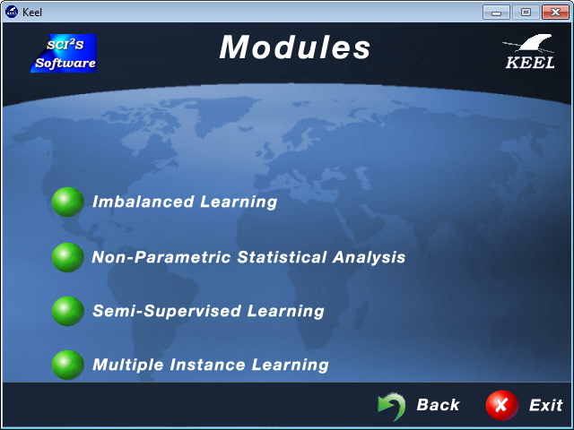
- Modules: This part includes new modules extending the
functionalities of the KEEL software suite for specific tasks associated
to the data mining process that require special treatment:
- Imbalanced Learning: This module features several algorithms specifically designed for Imbalanced Classification. The graphical interface gives the user access to a specific set of problems, algorithms and evaluation procedures covering the state-of-the-art in Imbalanced Classification maintaining the same structure and the same objectives as the Experiments section.
- Non-Parametric Statistical Analysis: This module provides the user with several Non-parametric Statistical procedures for pairwise (Wilcoxon test) and multiple comparisons (Friedman, Friedman Alligned, Quade and Contrast Estimation), together with several post-hoc procedures for advanced verification of results, given in raw CSV format. Furthermore, this module outputs all the results of the analyses in latex format, easing the inclusion of the reports obtained in any experimental report.
- Semi-Supervised Learning: This module, similar to the imbalanced learning module, is devoted to the creation and design of experiments related to semi-supervised learning. It features an interface similar to the experiments section featuring related datasets and methods which are useful in this scenario.
- Multiple Instance Learning: The multiple instance learning module, which follows the same scheme as the imbalanced and semi-supervised learning modules, allows the user to create and prepare experiments for multi-instance Learning. It features a graphical interface similar to the experiments section that gives access to specific multi-instance datasets and algorithms designed to tackle this problem.
These blocks that compose the KEEL Software Suite will also influence directly the organization of this User Manual. First of all, we will describe all the operations related to the Data Management section as a first step to obtain the data that is needed in the experiments. Then, the Experiments section is detailed and all of its operations are explained as the most powerful section of the suite. Next, the Educational section is presented and all its options are showed. Later, all the modules are presented in the same order as they appear in the KEEL Menu.
1.2 How to get KEEL
KEEL Software can be downloaded from the Web page of the project at http:www.keel.es/download.php. From here, several options are available:
- Download binary version of the latest prototype of the KEEL Software Suite, together with several related resources.
- Obtain the source code of the newest version of the prototype, which includes the implementation of all algorithms from the GitHub repository: https://github.com/SCI2SUGR/KEEL
- Select any of the former versions of the KEEL Software Suite, either the “.jar” files.
The simplest way to begin with KEEL is downloading the latest version of the prototype, which is already compiled for Java JRE 1.7 version. Additionally, all versions of the KEEL Software Suite include a basic package of datasets. However, we encourage users to browse through the KEEL-Dataset repository (http://www.keel.es/dataset.php), where more than 600 datasets (classification datasets, regression datasets and more) are available, ready to be imported to the prototype.
Once you have saved the compressed file with KEEL, you only need to unzip all files into any of your folders. Then, please place yourself into the “dist” folder and run the “GraphInterKeel.jar” file for the main menu.
Finally, just by following the guidelines provided in this document, you will be able to configure any data mining experiment. Furthermore, you might include your own algorithms for a more complete study. Please refer to the “KEEL Developer manual” for this purpose.
1.3 System requirements
KEEL is fully developed in Java. This means that any computer able to install and run a Java Virtual Machine (JVM) will be enough for running both the KEEL graphical interface and the data mining experiments created with the suite.
![]()
Currently, we recommend to install the latest stable version of Java (available at http://www.java.com/) although any JVM from the 1.7 version should be enough for running the graphical interface and the algorithms included in KEEL. Memory requirements (the only critical resource for some algorithms) can be adjusted when the experiments are created.
All these resources are free software, therefore, no custom or proprietary software is required to work with the tools provided by the KEEL project.
2 Getting Started
This section provides a quick introduction to using the KEEL software tool. The following subsections will allow you to download, install and run simple and elaborated examples in KEEL.
2.1 Download and Start KEEL
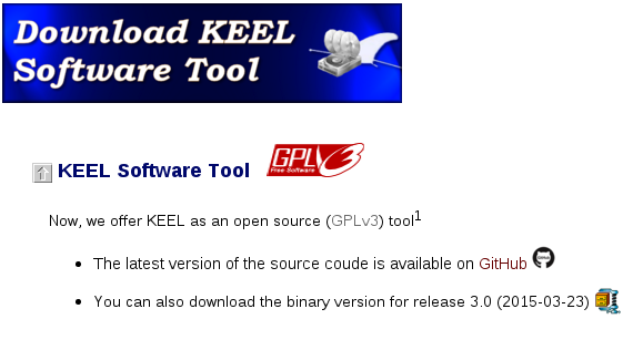
To follow along with this guide, first download the KEEL Software from the website (http:www.keel.es/download.php). You can either download the compiled version or the source code from the Git Repository (https://github.com/SCI2SUGR/KEEL). The figure below shows the two download options to get the last version of KEEL.
First, note that Java version 7 needs to be installed on your system for this to work. Depending on your computing platform you may have to download and install it separately. It is available for free from Sun GET JAVA. If you have Java already installed in your system, please, update it to the latest version if you want to use the newest KEEL versions.
2.1.1 Starting from the pre-compiled version
If you have downloaded the binary version (Software-20XX-YY-ZZ.zip), you first have to unzip this file. In order to launch the KEEL Software Suite, you just have to execute the GraphInterKeel.jar file. Then, navigate into dist folder, and run the program by simply execute the ”GraphInterKeel.jar” file. There are two different procedures to execute this jar file.
- Option 1: Right click on the jar icon by using the navigation utility of the OS
- Option 2: Execute the following command if you prefer to use a shell.
java -jar ./dist/GraphInterKeel.jar
Make sure you have properly setup the Java Path. For related issues, go to (https://www.java.com/en/download/help/path.xml).
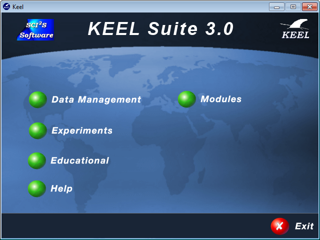
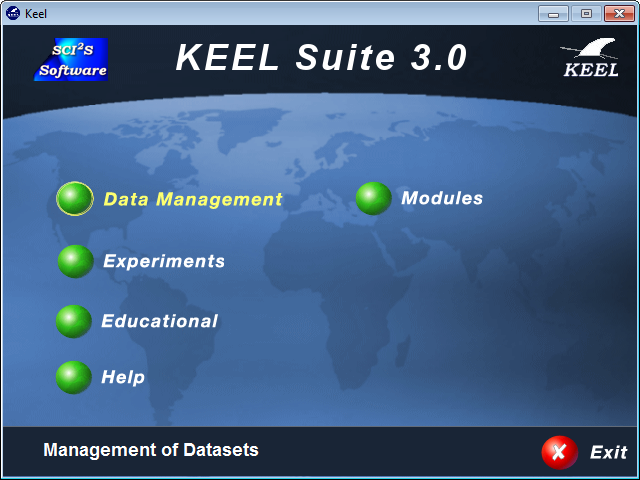
This is the launch window that appears after typing that command:
This GUI lets you importing datasets, run (educational) experiments, run different modules (Imbalanced Learning, Non-parametric Statistical Analysis, Semi-supervised learning and Multiple Instance Learning). It also provides a Help file with explaining the content of the initial screen.
2.1.2 Starting from the Source Code
If you want to compile KEEL source code it is advisable to use the Apache Ant Tool (available for download at the The Apache Ant Project web page: http://ant.apache.org/). The KEEL Software tool includes a ”build.xmlz” file to be used together with ant. To compile the KEEL project (assuming you have already installed ant) you just have to type the following commands:
ant cleanAll
This command erases previous binary files so that there aren’t any conflicts with new binary builts.
ant
This command builds the whole KEEL project binaries using the available source code. You can now navigate into the dist folder and run the generated .jar file:
java -jar ./dist/GraphInterKeel.jar
For more information, please refer to Subsection 1.2.
2.2 Importing your own data
The installation of new datasets into the application can be done using the Data Management module or the Experiments module. These modules can convert data from several formats (CVS, ARFF or plain text) to the KEEL format, thus allowing the user to quickly integrate them. In what follows, we show a simple example of use, enumarating the steps to be done. Please refer to Section 3.1 for full details.
Let’s say that we dispose of the following dataset file in CSV format that correspond to a subset of the Iris classification problem.
5.0,3.6,1.4,0.2,1
5.4,3.9,1.7,0.4,1
4.6,3.4,1.4,0.3,1
6.9,3.1,4.9,1.5,0
5.5,2.3,4.0,1.3,0
6.5,2.8,4.6,1.5,0
5.7,2.8,4.5,1.3,0
...
From the first screen:
- Click on Data Management.
- Import Data
- Since we only have a single file, we select ’Next’ in the section Import Dataset.
- Our format is CSV, so make sure that ’Select Input Format’ is set as: ’CSV to Keel’.
- Navigate and select your file. Press Next.
- KEEL will show you the translation performed.
- Let KEEL import your dataset to the Experiments Section. We will use it in the next section.
- Click on Save and put a name to the dataset (We denote it as ’example’).
- Select the type of problem. In this case, we will use Classification.
- You will have the option to edit the imported dataset, e.g. to put the name of variables. In this case, we will use this step to name the different characteristics as: sepalLength, sepalWidth, petalLength, petalWidth and class.
- KEEL will ask you to make partitions. For this example, we will click on Yes (k=10).
- We indicate the type of partition ”K-fold Cross Validation”, and Click on Divide.
After these steps, you will have created a new dataset with k-fold cross validation for the give CSV file. You can now close the current window and come back to the welcome KEEL’s screen.
2.3 An example of running experiments with KEEL
In this section, we present several examples on how to create and run experiments with the KEEL software tool. We will first present a simple example of an use case, and then, a more profound use case will be developed.
2.3.1 Standard use case
In this example, we will test the performance of one existing method within the KEEL software suite over the datasets that are already inserted in the tool. Specifically, we would like to obtain the accuracy performance of the C4.5 decision tree using a standard 10-fold cross validation partitioning scheme.
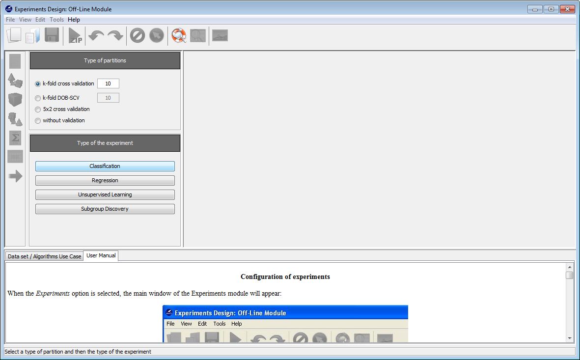
To do so, we will first select the “Experiments” option from the KEEL software suite main menu as show in Figure 7.

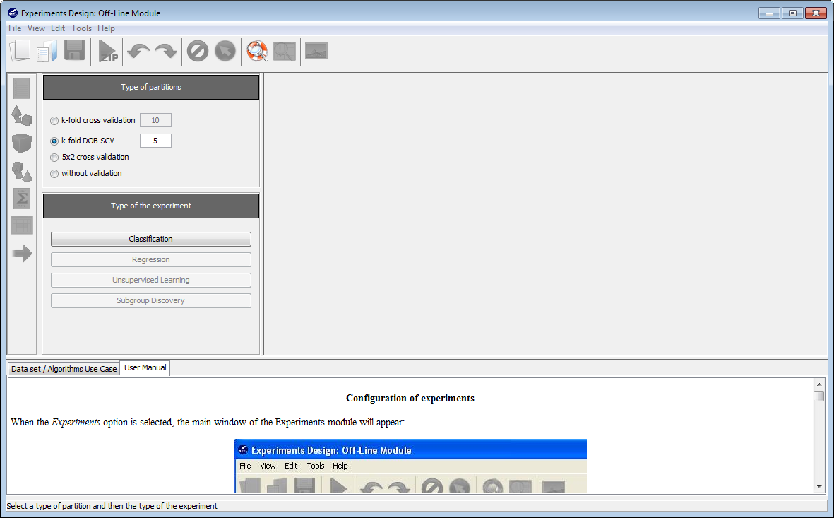
Now, we will select the type of experiment that we want to perform. First, we will select the partitioning scheme. As we want to perform a 10-fold cross validation, we need to select the first bullet “k-fold cross validation” from the “Type of partitions” menu, setting the value of k to 10. Then we will select the “Type of the experiment” clicking on the “Classification” button. This procedure is depicted in Figure 8.
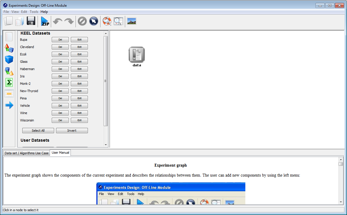
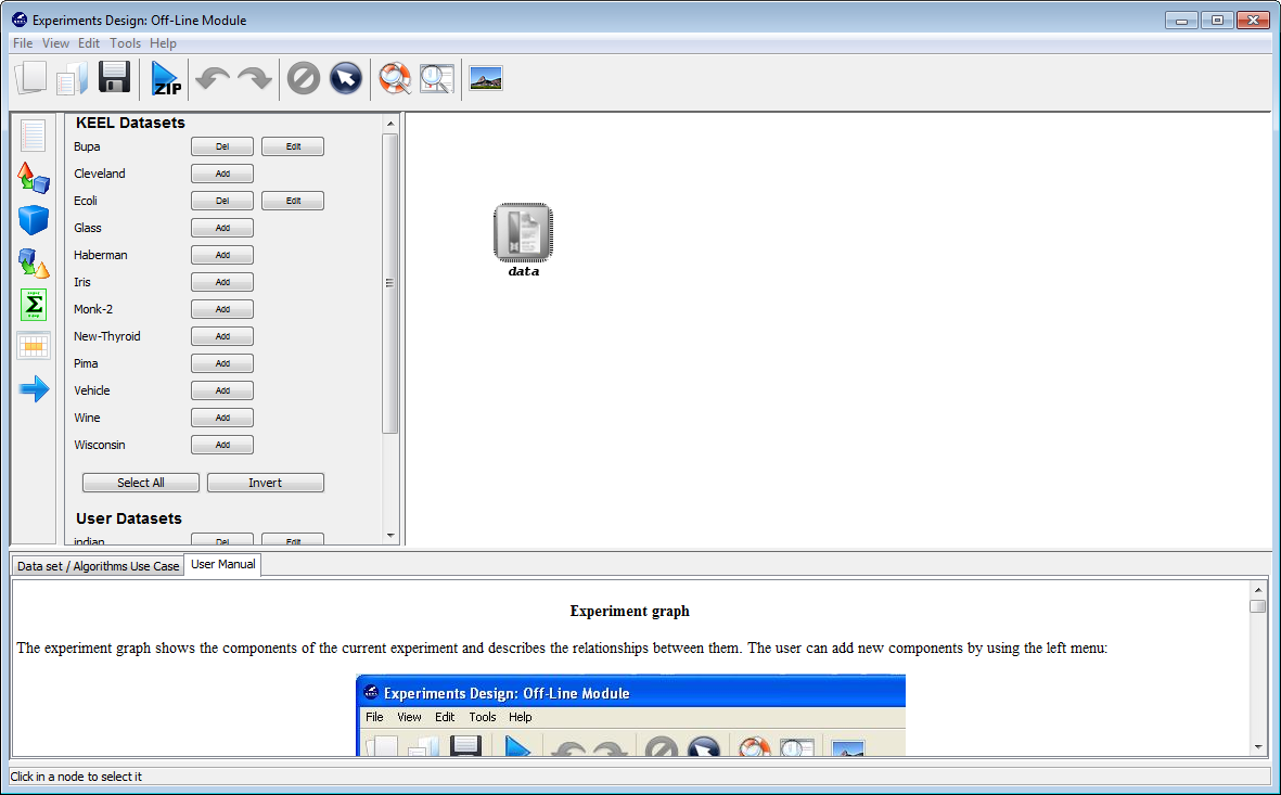
Now, we have to select the datasets that we want to use in this experiment. As we want to test all the data available in KEEL, we just click on the “Select All” button. This action will highlight all the datasets on the left panel. Then, we need to add these data to the experiment. To do so, we just have to click on any place of the right panel. Figure 9 shows how the KEEL screen has changed after adding the data to the experiment.
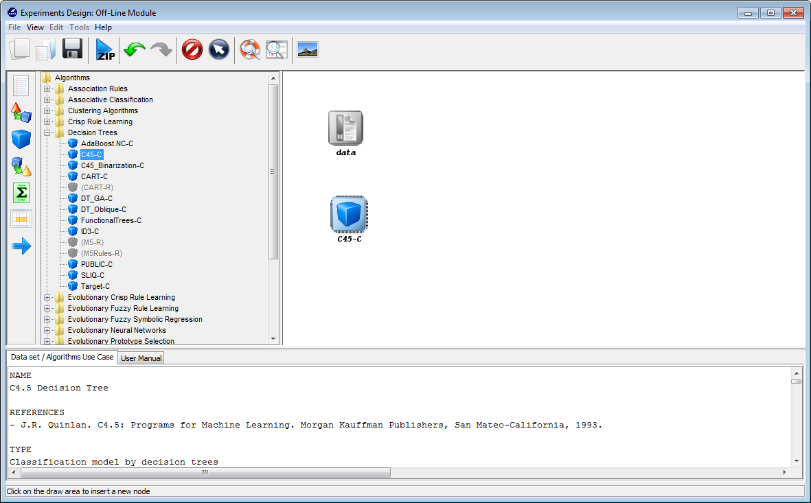
Now, we will select the methods that we want to add to the experiment. Since
we want to test the C4.5 decision tree, we click on the methods panel  on the
left side menu. This will prompt a list of methods organized by folders. We then
expand the “Decision Trees” folder, and click on the C45-C method, which is the
C4.5 decision tree that we want to use. Then, we click on any part of
the right panel to place this method in the experiments. If we want to
make sure that we have selected the correct method, we can click on the
“Data set / Algorithms Use Case” menu at the bottom to find further
information about the selected method. In our case, we check that “C45-C”
effectively corresponds with the “C4.5 Decision Tree” according to its
description. Figure 10 shows the screen used to add the C45-C method to the
experiment.
on the
left side menu. This will prompt a list of methods organized by folders. We then
expand the “Decision Trees” folder, and click on the C45-C method, which is the
C4.5 decision tree that we want to use. Then, we click on any part of
the right panel to place this method in the experiments. If we want to
make sure that we have selected the correct method, we can click on the
“Data set / Algorithms Use Case” menu at the bottom to find further
information about the selected method. In our case, we check that “C45-C”
effectively corresponds with the “C4.5 Decision Tree” according to its
description. Figure 10 shows the screen used to add the C45-C method to the
experiment.
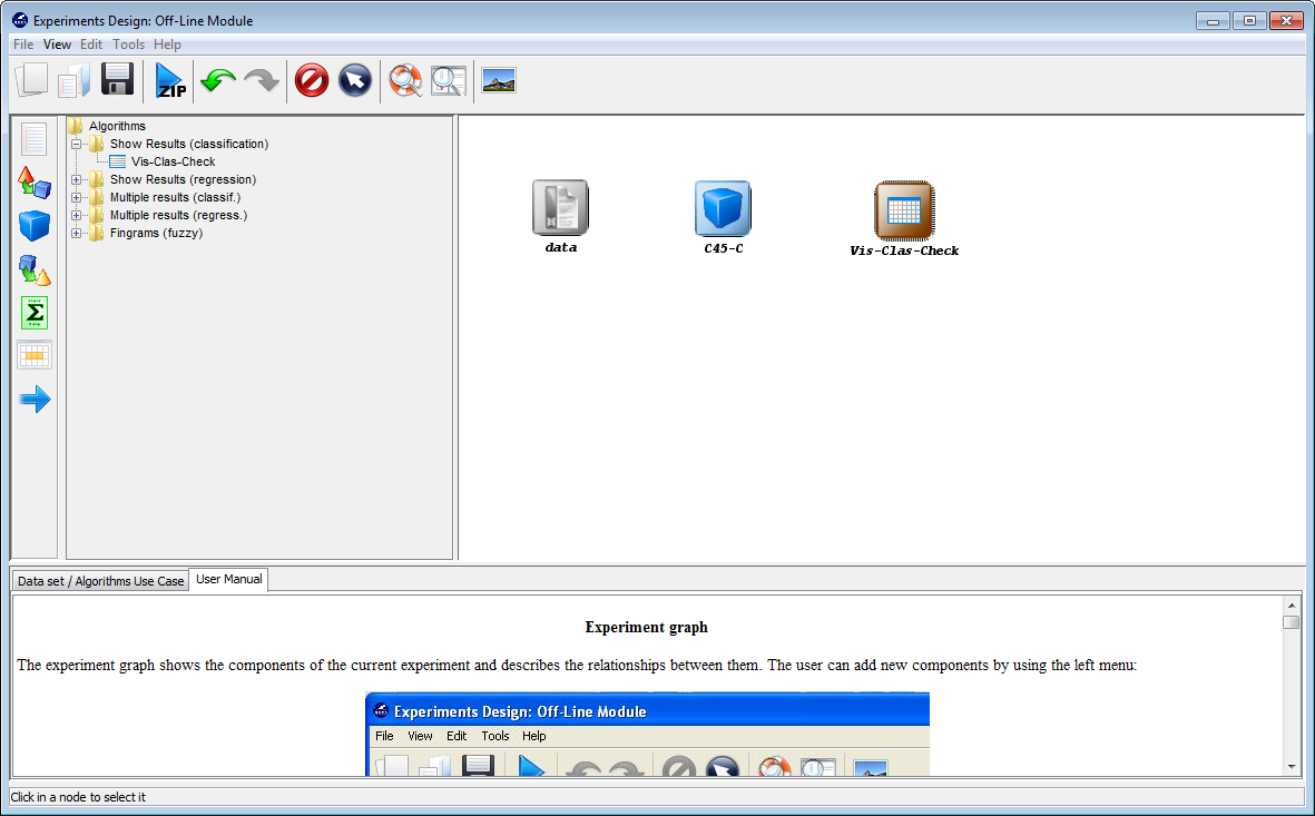
Furthermore, we want to test the accuracy obtained by this method. To easily
check the accuracy obtained by the C4.5 decision tree, we want to include a
visualization method. To do so, we click on the visualization panel  on the
left side menu. This will prompt a list of methods organized by folders. Since we
are using a single classification method, we expand the “Show Results
(classification)” folder and select its only method “Vis-Class-Check”. Now, we
click on any part of the right panel to place this visualization approach in the
experiment. Figure 11 shows how the visualization method is added to the
experiment.
on the
left side menu. This will prompt a list of methods organized by folders. Since we
are using a single classification method, we expand the “Show Results
(classification)” folder and select its only method “Vis-Class-Check”. Now, we
click on any part of the right panel to place this visualization approach in the
experiment. Figure 11 shows how the visualization method is added to the
experiment.
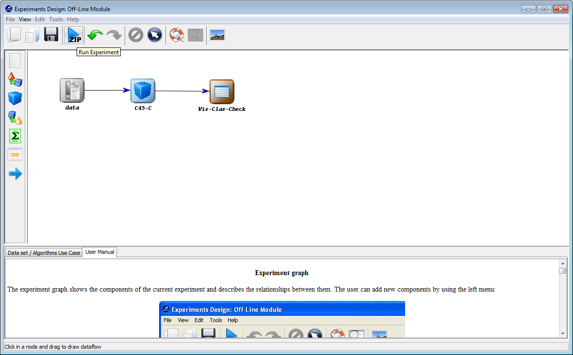
Now we need to establish the execution flow of the experiment. In this case,
we just need to connect the data, with the method and with the visualization
approach. To do so, we click on the arrow (connection)  on the left side menu.
Then, we connect the “data” and “C45-C” elements, clicking on the first one and
dragging the click to the second one. We repeat this action with “C45-C”
and “Vis-Clas-Check”. Figure 12 displays the current state of the KEEL
screen.
on the left side menu.
Then, we connect the “data” and “C45-C” elements, clicking on the first one and
dragging the click to the second one. We repeat this action with “C45-C”
and “Vis-Clas-Check”. Figure 12 displays the current state of the KEEL
screen.

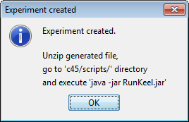
Finally, we click on the generate ZIP experiment button on the top menu  (Figure 13). This will prompt the generation of the zip experiment. A menu will
be shown to select where we want to place our experiment and how we want to
name it. We select the name “c45” and we place the ZIP file in the “D:\\” folder.
We have now created our KEEL experiment!
(Figure 13). This will prompt the generation of the zip experiment. A menu will
be shown to select where we want to place our experiment and how we want to
name it. We select the name “c45” and we place the ZIP file in the “D:\\” folder.
We have now created our KEEL experiment!
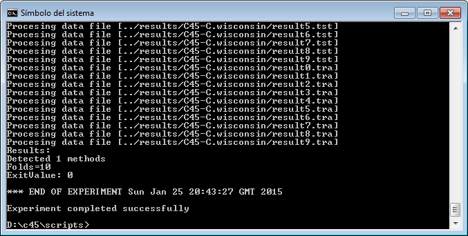
However, we have not finished yet as we have to run the experiment. We now unzip the “c45.zip” that has just been generated. We move to its “scripts” subfolder and type in a console “java -jar RunKeel.jar”. With this command, we launch the experiment. Now we wait until the experiments are completed; this is shown with the message “Experiment completed succesfully” (Figure 15). We have now finished running our KEEL experiment!
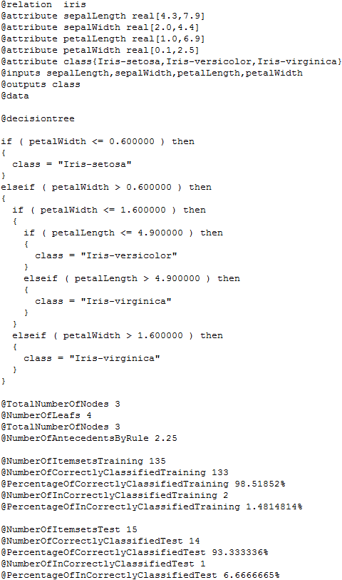
If we want to explore the results we have obtained, we have to check the contents of the “results” subfolder associated to our KEEL experiment. In this subfolder we can find several subfolders containing all the results. The “C45-C.datasetName” subfolders contain the detailed results of the C4.5 algorithm over the “datasetName” dataset. In each of these subfolders, we will find 30 files, 3 per each partition, one .tra file, containing the classification results of the training partition, one .tst file, containing the classification results of the test partition, and one .txt file, containing the built tree and related statistics. Figure 16 shows the content of one of these .txt files for the “iris” dataset.
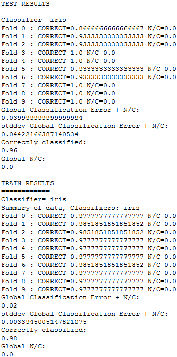
Moreover, in the “results” subfolder, we can find an additional subfolder named “Vis-Clas-Check”. This folder contains the summary results of the C4.5 algorithm considering the accuracy. Specifically, we will first see another subfolder named “TSTC45-C”, and in it, the .stat files with the accuracy associated to each dataset. Figure 17 shows the content of one of the .stat file associated to the “iris” dataset.
2.3.2 Advanced use case
In this example, we will test the performance of two existing methods within the KEEL software suite over some datasets and we will compare them to see which method performs better through the use of statistical tests. Specifically, we would like to compare the classification accuracy performance of an SMO support vector machine against the K-nearest neighbor classifier (from the lazy learning family) using the 5-fold DOB cross validation partitioning scheme and comparing some datasets which are not initially including in the tool: one from the KEEL dataset repository and the other one from the UCI dataset repository.
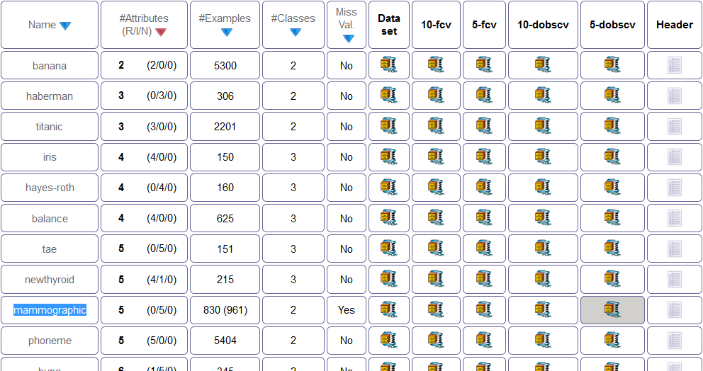
To perform this experiment, the first step would be the obtaining of these external datasets. We are going to use the “mammographic” classification dataset from KEEL dataset repository. To download this data, we access the associated webpage in its standard classification section through http://www.keel.es/category.php?cat=clas. As partitions are available for this data, we download the generated partitions for 5-dobscv, as seen in Figure 18. We unzip the downloaded file.
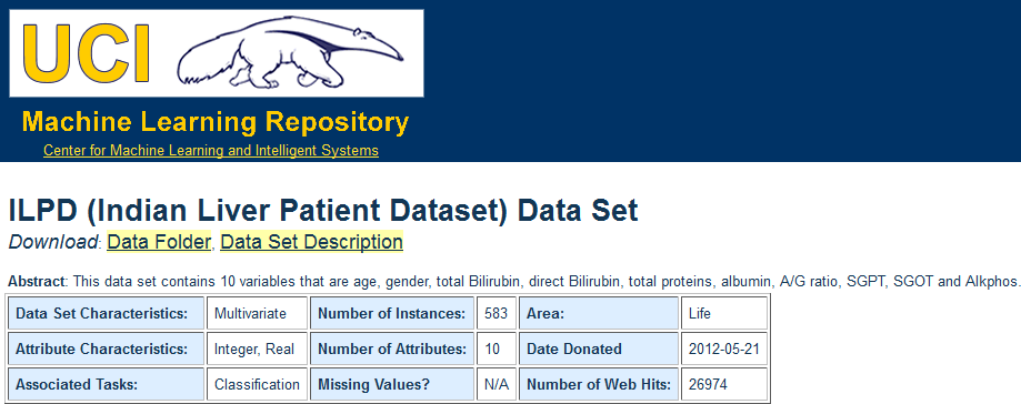
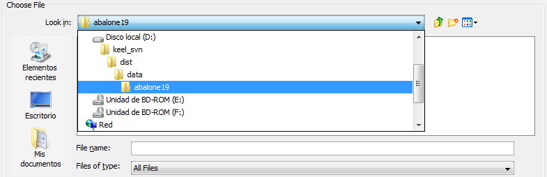
Moreover, we are also going to use the “Indian Liver Patient Dataset” (ILPD) dataset from the UCI dataset repository. We access the repository through http://archive.ics.uci.edu/ml/index.html and we download the dataset, as seen in Figure 19. As the only available format is CSV, we obtain this format and we will process the file with KEEL.
Now, we start the KEEL software suite. We will select the “Data Management” option from the KEEL software suite main menu as show in Figure 20.
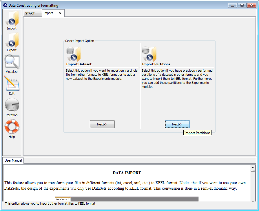
Since we are going to add datasets, we select the “Import Data” option from the menu as seen in Figure 21.
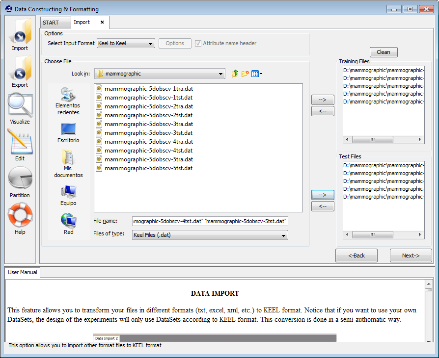
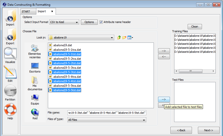
To add the “mammographic” dataset we will select the “Import Partitions” option (Figure 22), as we downloaded a set of partitions for this data. In the following screen (Figure 23), we have to select the location where we unzipped the downloaded files and organize considering if they are training or test files. Moreover, we need to specify that the data files are originally in DAT format, selecting “Keel to Keel” in the “Select Input Format” option.
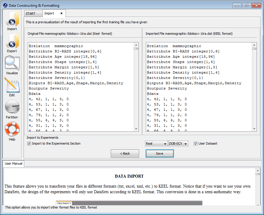
Before finally adding this dataset to KEEL, we find another confirmation window (Figure 24) where we need to include additional information about the data we are including. First, we need to make sure that the “Import to the Experiments Section” checkbox is on. Then, we need to select the type of dataset and partitioning of the data we are adding. In this case, we will use the options “Real” and “DOB-SCV” respectively. We will then click on the “Save” button.
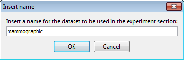
Then, a dialog asks to provide a name for the dataset (Figure 25). We select “mammographic” and confirm this selection. Then, we are asked about the type of problem this dataset belongs to (Figure 26) where we select “Classification”. Now we have successfully imported the “mammographic” dataset.

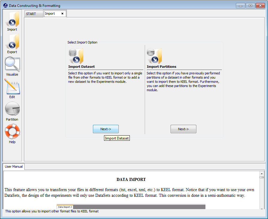
Now we are back to the “Import Data” menu. Since we do not have partitions for the “Indian Liver Patient Dataset” (ILPD), we select the “Import Dataset” option now (Figure 27).
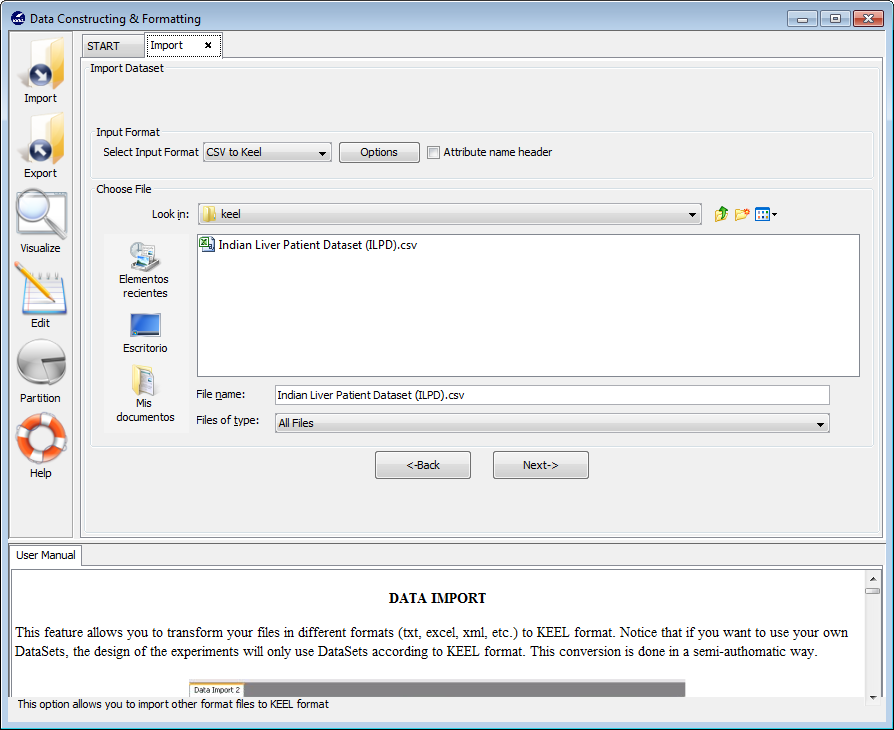
In the first screen that is shown, Figure 28), we have to search for the input file that contains the whole dataset and select it. We also need to include some information about the data in the “Input Format” section. Specifically, we have to select the “CSV to Keel” option and untick the “Attribute name header” option as the first line in the CSV file does not contain any information about the attributes. Having selected all the options, we click on the “Next” button.
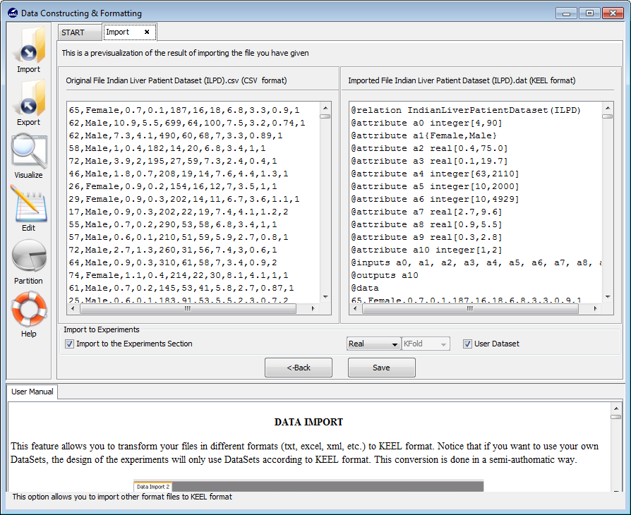
Now, we find a confirmation window (Figure 29) where we need to include additional information about the data we are including. As in the previous case, we need to make sure that the “Import to the Experiments Section” checkbox is on. Then, we need to select the type of dataset we are adding which in this case will be “Real”. We will then click on the “Save” button.
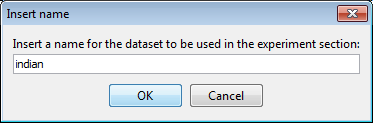
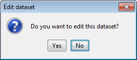
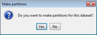
We will now be asked by a dialog (Figure 30) the name of this dataset. We select “indian” and confirm this selection. Then, we are asked about the type of problem this dataset belongs to (Figure 31) where we select “Classification”. Next, we are asked whether we want to edit this dataset (Figure 32) where we answer “No” as we do not want to perform changes to the original dataset. Afterwards, we are asked if we want to perform partitions to this dataset (Figure 33). In this case, we answer “Yes” as we want to perform experiments with DOB-SCV.

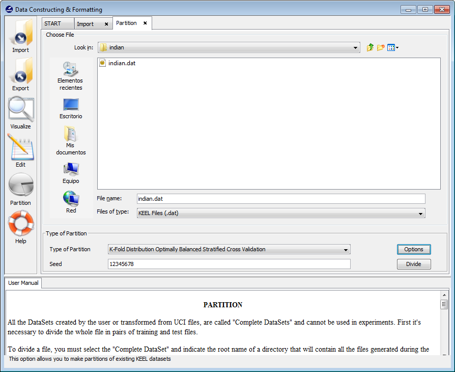
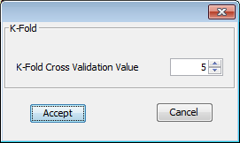
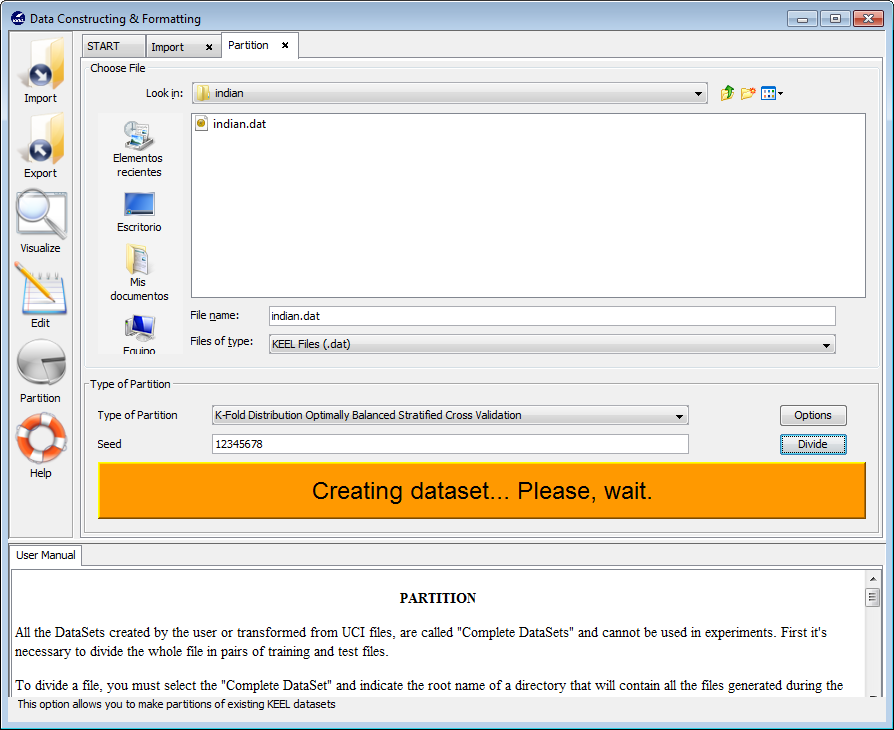
We are now at the partitioning scheme (Figure 34). We have to select the options for the partitioning of our data. In our case, we first select the “Indian Liver Patient Dataset” dataset selecting the “indian.dat” file. Then, we select the correct “Type of Partition” by selecting the “K-Fold Distribution Optimally Balanced Stratified Cross Validation” option from the list. Additionally, we have to click on the “Options” button to change the number of k fold to 5 (Figure 35). Having selected the appropriate options we now click on the “Divide” button.
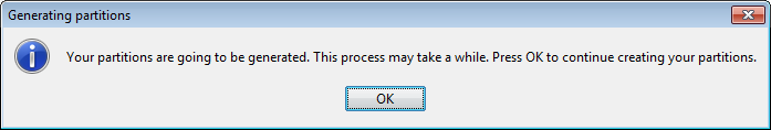
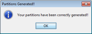
First of all we obtain a message stating that this process may be long (Figure 36). We click on it and wait for the partitions to be created (Figure 37). When they are created we receive a message with that information (Figure 38). We can now go back to KEEL main menu.
As we have added our data now we will select the “Experiments” option from the KEEL software suite main menu as show in Figure 39.
Now, we will select the type of experiment that we want to perform. First, we will select the partitioning scheme. As we want to perform a 5-fold DOB cross validation, we need to select the second bullet “k-fold DOB-SCV” from the “Type of partitions” menu, setting the value of k to 5. Then we will select the “Type of the experiment” clicking on the “Classification” button. This procedure is depicted in Figure 40.
Now, we have to select the datasets that we want to use in this experiment. We have available the datasets that we have just added to KEEL under the “User Dataset” listing. We select the “indian” and “mammographic” datasets. We also select the “Bupa” and “Ecoli” datasets from the “KEEL Datasets” listing. Now, we need to add these data to the experiment. To do so, we just have to click on any place of the right panel. Figure 41 shows how the KEEL screen has changed after adding the data to the experiment.
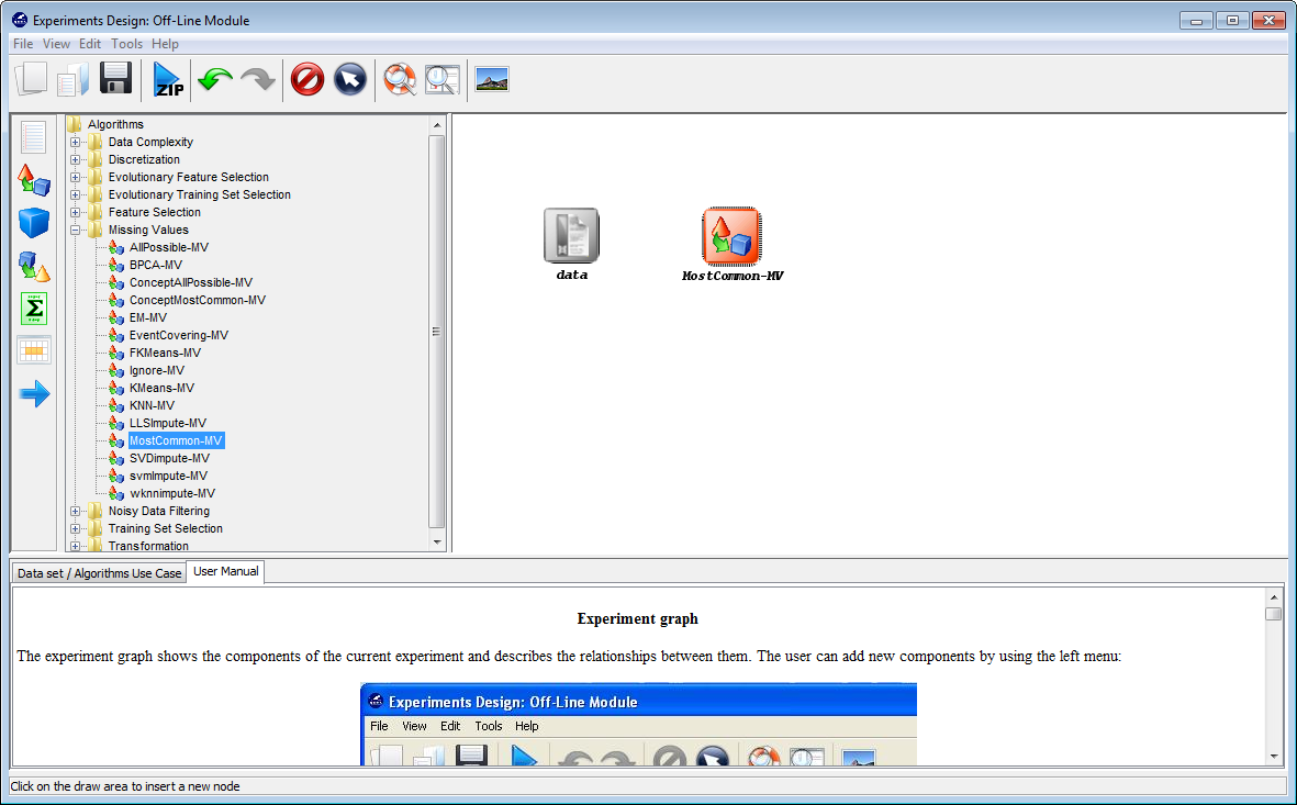
Now, we will select the methods that we want to add to the experiment. Since
the data that we have contains some missing values, we will introduce a
preprocessing method to imputate the missing values. To do so, we click on the
pre-processing panel  on the left side menu. This will prompt a list of
pre-processing approaches organized by folders. We then expand the
“Missing Values” folder, and click on the MostCommon-MV method,
which is the missin values method that we want to use. Then, we click
on any part of the right panel to place this method in the experiments.
Figure 42 shows the screen including the mentioned missing values
approach.
on the left side menu. This will prompt a list of
pre-processing approaches organized by folders. We then expand the
“Missing Values” folder, and click on the MostCommon-MV method,
which is the missin values method that we want to use. Then, we click
on any part of the right panel to place this method in the experiments.
Figure 42 shows the screen including the mentioned missing values
approach.
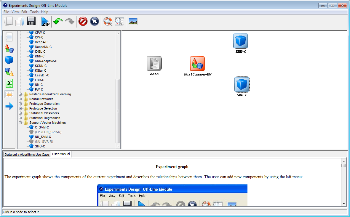
As we want to compare two classifiers, we click on the methods panel on
the left side menu. This will prompt a list of methods organized by folders. We
then expand the “Lazy Learning” and “Support Vector Machines” folders as they
contain the methods we want to test. We click on the “KNN-C” method in the
“Lazy Learning” folder and then on any part of the right panel to place this
method in the experiments. Then, we do the same with the “SMO-C” method in
the “Support Vector Machines” folder. Figure 43 shows the screen representing
the experiment.
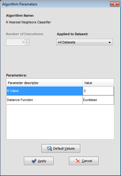
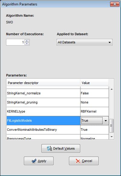
We may want to change the parameters associated to the methods. To do so, we just have to double-click on top of the box containing the method whose parameters we want to change. We double-click on the “KNN-C” method and a new menu is opened (Figure 44). In there, we modify the “K Value” to 3, using the 3 nearest neighbors to classify. Then, we double-click on the “SMO-C” algorithm and a new menu is opened (Figure 45). As we want to change the kernel for the support vector machine and its option to fit the logistic models, we change the option “KERNELtype” to “RBFKernel” and “FitLogisticModel” to “True”.
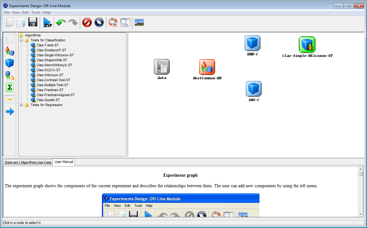
Furthermore, we want to test the accuracy obtained by these methods. We first
want to compare the methods performance according to a statistical test. Since
we are comparing two approaches, we will use the Wilcoxon test. Therefore, we
click on the statistical test panel  on the left side menu, and expand the “Tests
for Classification” folder as we are performing a classification experiment.
Among the methods, we select the Wilcoxon test which is named as
“Clas-Wilcoxon-ST” and we click on the right panel to place this test. Figure 44
shows the current state of the experiment.
on the left side menu, and expand the “Tests
for Classification” folder as we are performing a classification experiment.
Among the methods, we select the Wilcoxon test which is named as
“Clas-Wilcoxon-ST” and we click on the right panel to place this test. Figure 44
shows the current state of the experiment.
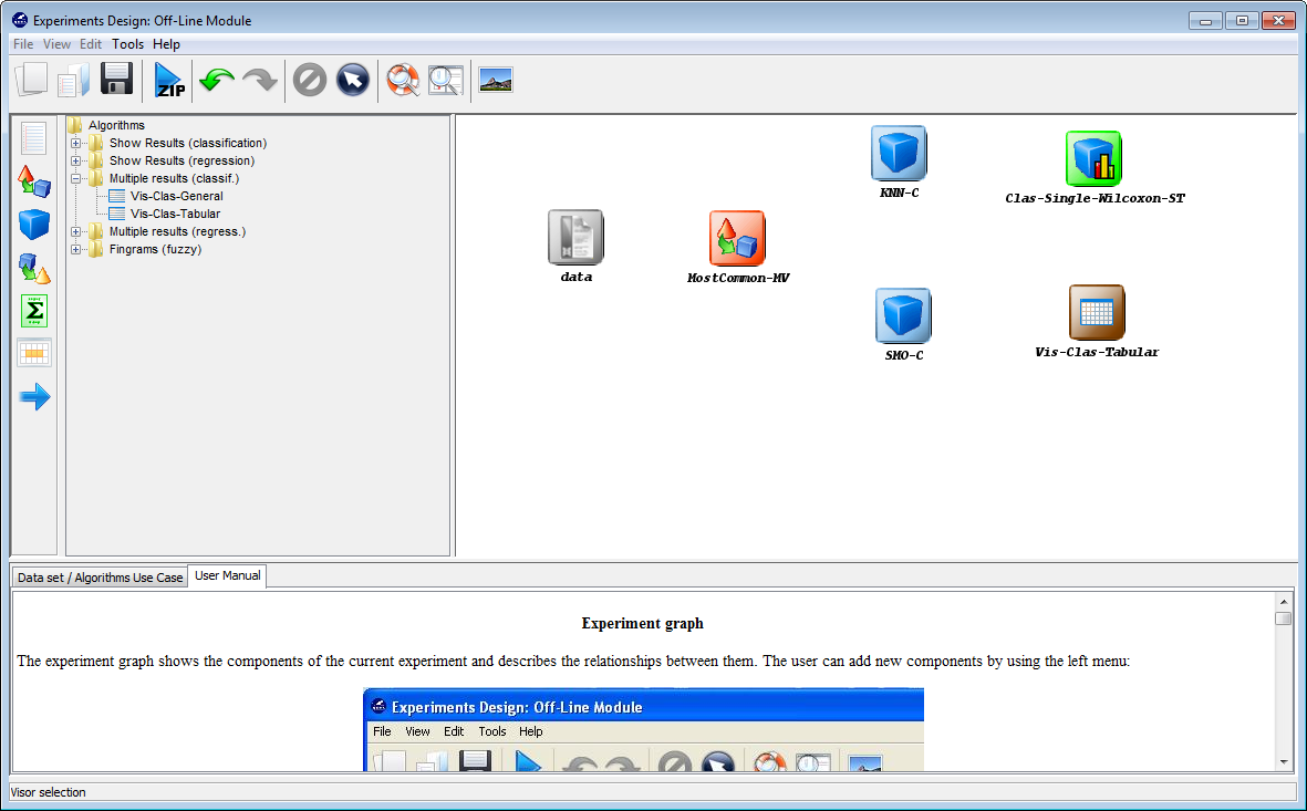
Moreover, we also want to obtain statistics about the accuracy obtained by the
tested methods. To calculate this information we will include a visualization
method clicking on the visualization panel on the left side menu. This will
prompt a list of methods organized by folders. Since we are using several
classification methods, we expand the “Multiple results (classif.)” folder and
select one of its methods “Vis-Class-Tabular”, which will organize the
information in tables. Now, we click on any part of the right panel to place this
visualization approach in the experiment. Figure 47 shows how the visualization
method is added to the experiment.
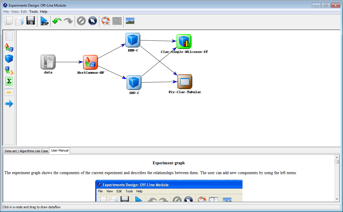
Now we need to establish the execution flow of the experiment. In this case,
we need to connect the data, with the preprocessing method, then with
the classification methods, and then both methods will be connected
with the statistical test and the visualization approach. To do so, we
click on the arrow (connection) on the left side menu. Then, we
connect the “data” and “MostCommon-MV” elements, clicking on the
first one and dragging the click to the second one. We repeat this action
with “MostCommon-MV” and “KNN-C”, “MostCommon-MV” and
“SMO-C”, “KNN-C” and “Clas-Single-Wilcoxon-ST”, “KNN-C” and
“Vis-Clas-Tabular”, “SMO-C” and “Clas-Single-Wilcoxon-ST” and “SMO-C”
and “Vis-Clas-Tabular”. Figure 48 depicts the current state of the KEEL
screen.
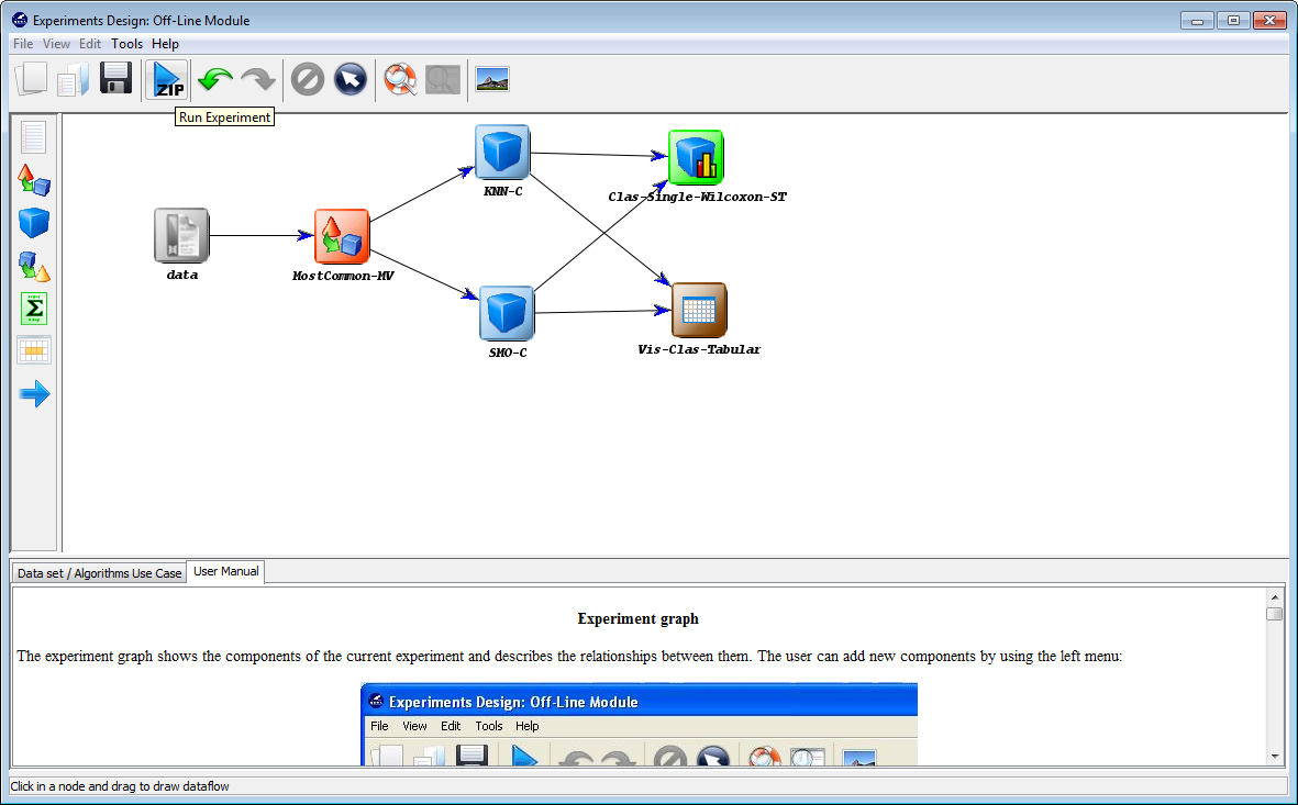
Finally, we click on the generate ZIP experiment button on the top menu
(Figure 49). This will prompt the generation of the zip experiment. A
menu will be shown to select where we want to place our experiment
and how we want to name it. We select the name “knnvssmo” and we
place the ZIP file in the “D:\\” folder. We have finally created our KEEL
experiment!!!
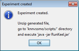
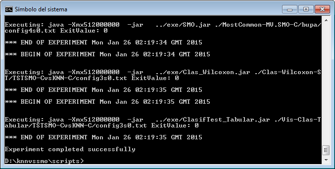
However, we have not finished yet as we have to run the experiment. We now unzip the “knnvssmo.zip” that has just been generated. We move to its “scripts” subfolder and type in a console “java -jar RunKeel.jar”. With this command, we launch the experiment. Now we wait until the experiments are completed; this is shown with the message “Experiment completed succesfully” (Figure 51). We have now finished running our KEEL experiment!
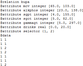
Now we would like to explore the results that we have obtained. To do so, we have to check the contents of the “results” subfolder associated to our KEEL experiment. In this subfolder we can find several subfolders containing all the results. First, we find a set of subfolders with names like “KNN-C.datasetName” or “SMO-C.datasetName”. These subfolders contain the detailed results of the KNN and SMO algorithms over the “datasetName” dataset. In each of these subfolders, we will find 10 files, 2 per each partition, one .tra file, containing the classification results of the training partition, one .tst file, containing the classification results of the test partition. Figure 52 shows the content of one of these .tra files for the “bupa” dataset using the KNN algorithm.
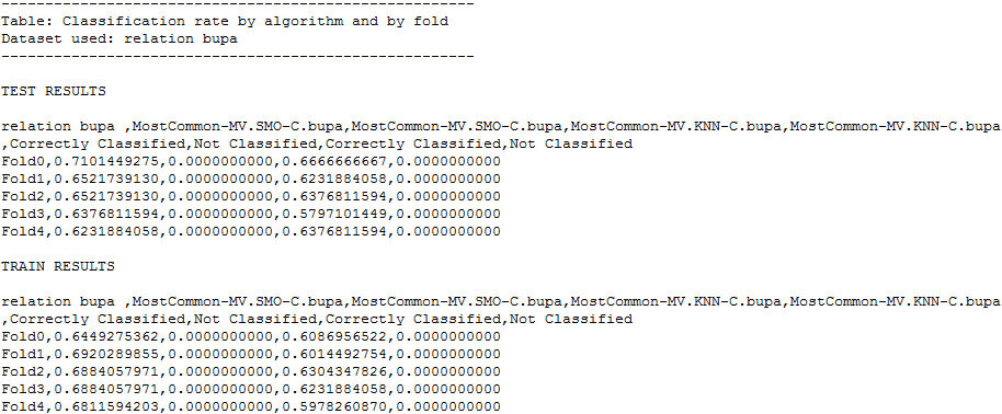
Moreover, in the “results” subfolder, we can find an additional subfolder named “Vis-Clas-Tabluar”. This folder contains the summary results of both KNN and SMO algorithms considering the accuracy. Specifically, we will first see another subfolder named “TSTSMO-CvsKNN-C”, and in it, the .stat files with the accuracy associated to each dataset. For instance, the “Summary_s0.stat” file, shows a table with the average statistics of all the methods; the “datasetName_KNN-C_ConfussionMatrix_s0.stat” shows the confusion matrix for the “datasetName” dataset for the “KNN-C” method; and the “datasetName_ByFoldByClassifier_s0.stat” show a table with the accuracy obtained in each fold by the methods for the “datasetName” dataset. Figure 17 shows the content of one of the .stat file associated to the “iris” dataset.
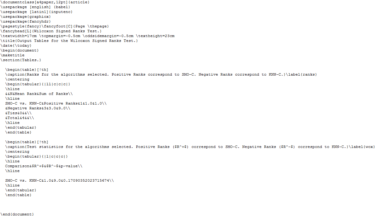
Furthermore in the “results” subfolder, we can find another additional subfolder named “Clas-Wilcoxon-ST”. This folder contains the results associated to the Wilcoxon statistical test. Specifically, we will first see another subfolder named “TSTSMO-CvsKNN-C”, and in it, several .stat files and a .tex file. The .stat files include the information associated to the Wilcoxon test of each used dataset. The .tex file is a LATEXfile providing the output of the Wilcoxon test over all the selected datasets. Figure 54 shows the content of one of the “output.tex” file.
2.4 Where to go from here
Congratulations on running your first experiments with KEEL!
For an in-depth overview of the KEEL features, go into the further sections to:
- Manage your data: Import, export, conversion between file formats, visualize data, edit data, and data partition (Section 3)
- Design more elaborated experiments (Section 4).
- Get a better understanding about how to run experiments (Section 5).
- Design on-line education experiments (Section 6).
- Design specific experiments within the different modules: Modules Imbalanced learning, Semi-supervised learning and Multiple instance learning (Section 7).
3 Data Management
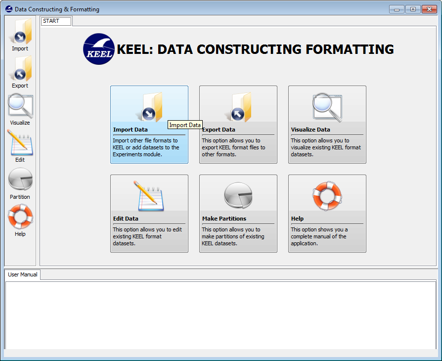
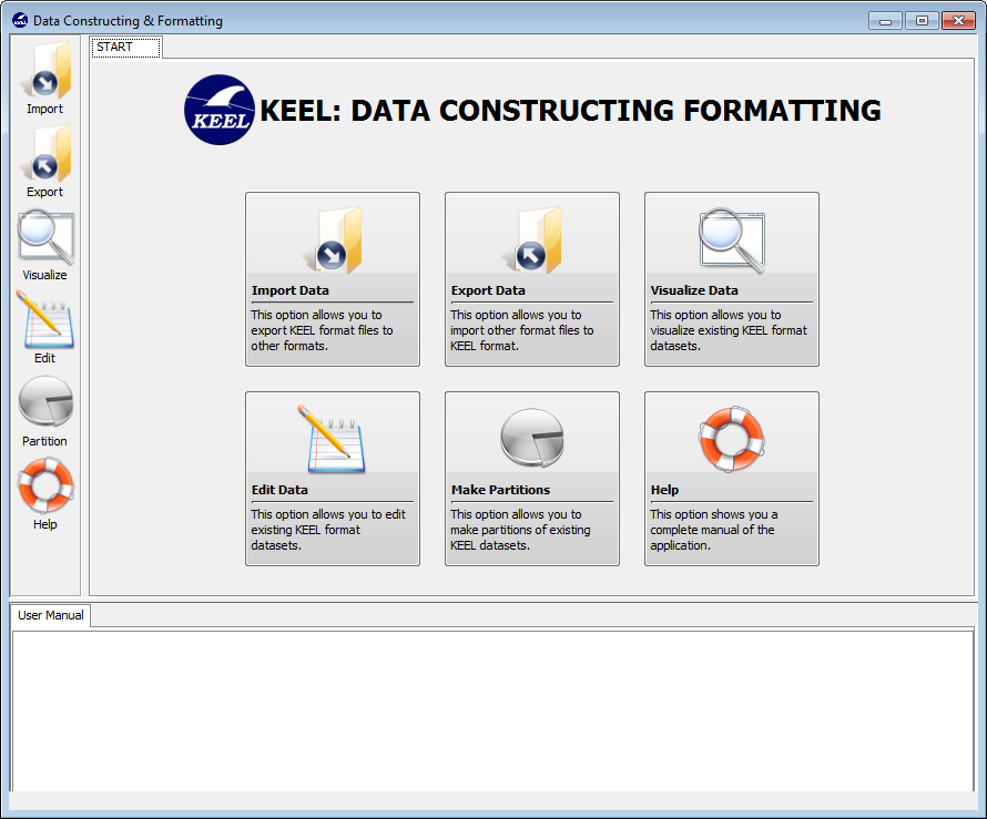
The next tasks are possible to be carried out using KEEL data management module. In Figure 3, the data management main menu is shown featuring the available options:
- Import Data: This option allows a user to export KEEL format files to other formats.
- Export Data: This option allows a user to import other format files to the KEEL format.
- Visualize Data: This option allows a user to visualize existing KEEL format datasets.
- Edit Data: This option allows a user to edit existing KEEL format datasets.
- Make Partitions: This option allows a user to make partitions for existing KEEL datasets.
3.1 Data import
The import option allows a user to transform files in different formats (TXT, Excel, XML, etc.) to the KEEL format. Notice that if you want to use your own datasets within the KEEL software suite, the design of the experiments will only use datasets according to the KEEL format, therefore, a previous step of import will be required.
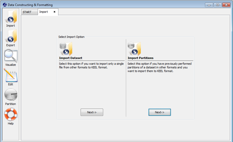
Figure 56 shows the two possible options to import datasets. One option consists of importing one dataset, the other option consists of importing a set of partitions which you have available in other formats different to the KEEL format. In the following, we show the process of both options.
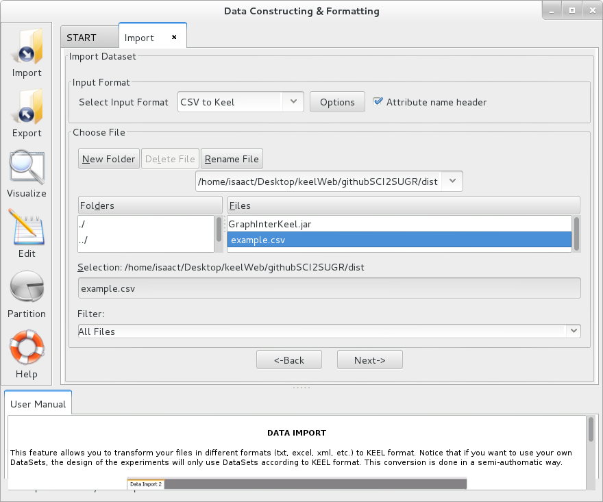
3.1.1 Import dataset
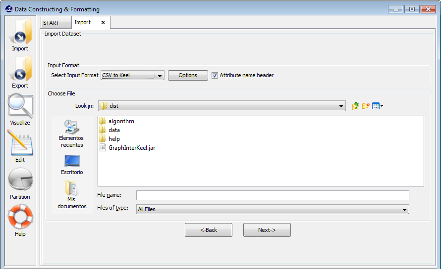
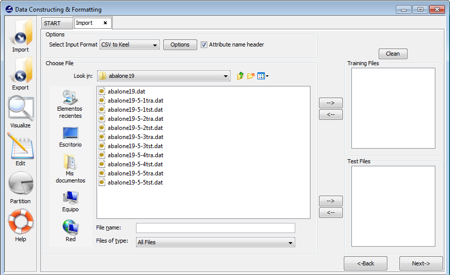
Select this option if you want to import only a single file from other formats to KEEL format. Figure 57 shows the window to this option.
To import a dataset, it is necessary to follow the next steps:
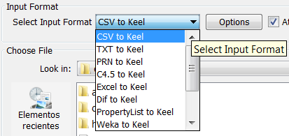
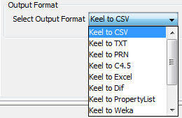
- Step 1. Select Input Format. First of all, you must select the source file
format of the dataset. The formats admitted are CVS, TXT, PRN, C4.5,
Excel, DIF, PropertyList and Weka. The different options are shown in
Figure 58.
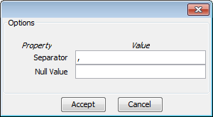
The Options button allows you to configure if it is necessary a certain separator and null value used in the source file, as shown in Figure 59.
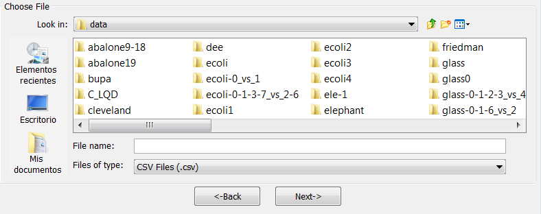
- Step 2. Select the source file. After specifying the file format used in source
file, the path of this file must be specified (see Figure 60). A browser
commonly known from many other GUI programs is used to define this
path.
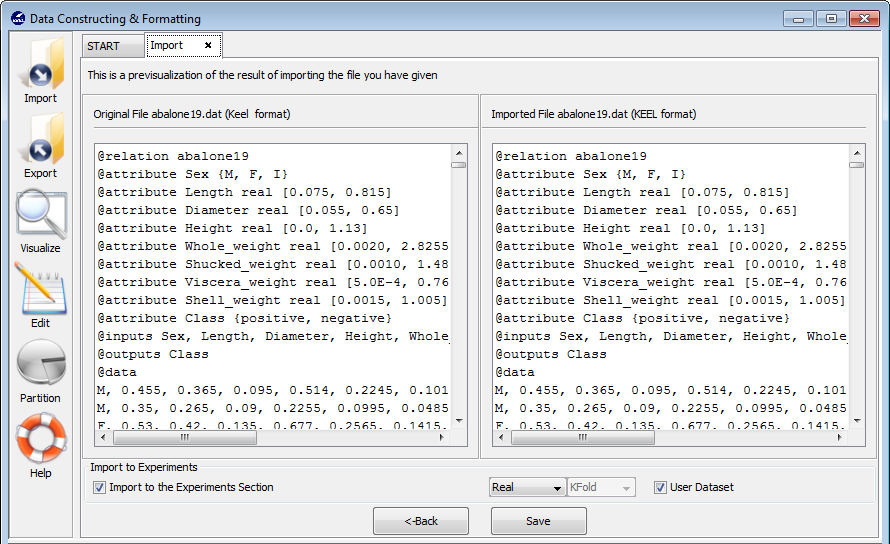
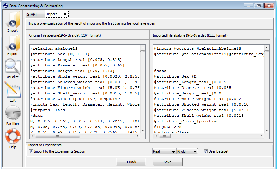
- Step 3. Save the files. Once the type of conversion and the source file have
been configured, you must click Next button and then, the original and the
imported file are shown (see Figure 61).
If you agree with the conversion done, there are two options to save the imported file (Figure 61):
- Check the Import to the experiments section: if you mark this option and click the Save button, the dataset converted will be included as option in the KEEL experiments. This dataset will be available to execute with the methods of KEEL.
- Uncheck the Import to the experiments section: if you do not select this option, when you click the Save button, you have to select the destination directory for the transformed dataset.
Finally, the tool will ask if you agree to perform data partitions for this new dataset. For this procedure, please refer to Section 3.6 (Data partitions) in this document.
3.1.2 Import partitions
Select this option if you have previously performed partitions of a dataset in other formats and you want to import them to KEEL format. This option allows the selection of a set of training and test files separately. Figure 62 shows the window with respect to this option.
To import partitions, it is necessary the next parts:
- Step 1. Select Input Format. First of all, you must select the source
file format of the dataset. The formats admitted are CVS, TXT, PRN,
C4.5, Excel, DIF, PropertyList and Weka. The different options were
shown in Figure 58.
The Options button allows you to configure if it is necessary a certain separator and null value used in the source file (as shown in Figure 59).
- Step 2. Select the source file. After specifying the file format used in
source file, the path of this file must be specified. You have to use the
arrows to include the files in training or test properly (see Figure 63).
- Step 3. Save the files. Once type of conversion and source file have been
configured, you must click the Next button and the original and the
imported file are shown (see Figure 64).
If you agree with the conversion done, there are two options to save the imported file:
- Check the Import to the experiments section: if you mark this option, two new options are available. With this option you configure if the dataset is a real or laboratory dataset and the partitions that you are used. Three partitions are applicable: k-fold, 5x2 or DOB-SCV cross validation. Then, when you select the Save button, the dataset that you are converted will be included as option in the KEEL experiments.
- Uncheck the Import to the experiments section: if you do not select Import to the experiments section, when you click the Save button, you have to select the destination directory for the transformed datasets.
3.1.3 Importing SQL databases to KEEL format
This section describes how to import databases stored in SQL format to KEEL format.
Once the Import Dataset option have been chosen within the Import menu, it is necessary to follow the next steps:
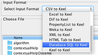
- Step 1. Select Input Format. First of all, you must select the source
file format of the dataset, which in this case is Database SQL to KEEL
(Figure 65).
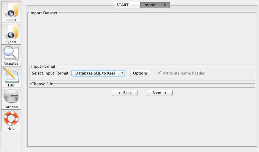
- Step 2. Select the parameters for the SQL database. After specifying the
file format used (SQL databases), the window shown in Figure 66
appears.
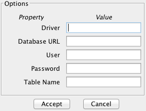
Then, the parameters to access the database must be specified. The Options button allows you to configure these parameters (see Figure 67). The meaning of these parameters is the following:
- Driver. The name of the Java driver that is needed in order to access to the SQL database. KEEL incorpores the driver com.mysql.jdbc.Driver by default, so we can use this to fill the field.
- Database URL. The URL of the database specified in the format jdbc:mysql://server:port/database, where server is the name or address of the server, port is the port of connection and database is the name of the database in which the SQL table is stored. For example, in order access to a local database called test, we can specify the Database URL as jdbc:mysql://localhost:3306/test.
- User and Password. They are the user name and password required to access to the database specified in the previous field, Database URL.
- Table Name. The name of the table that we want to convert to KEEL format.
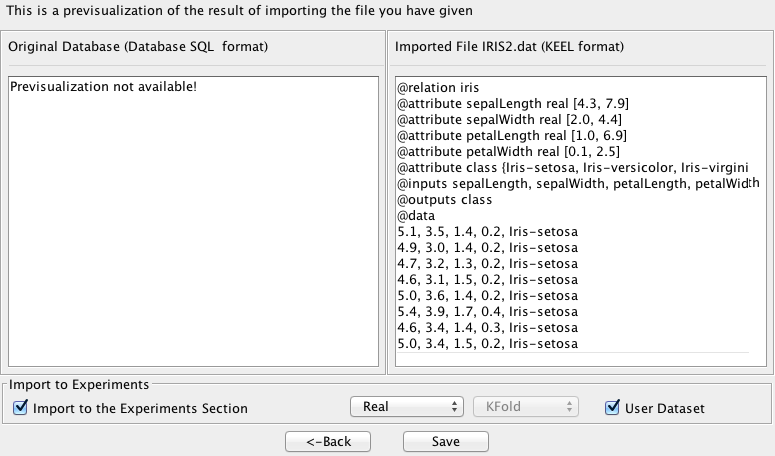
- Step 3. Save the files. Once the type of conversion and the source file have
been configured, you must click Next button and then, the original (in this
case, it will be in blank) and the imported file are shown (see Figure
68).
Finally, like in any other dataset importation, if you agree with the conversion done, there are two options to save the imported file:
- Check the Import to the experiments section: if you mark this option and click the Save button, the dataset converted will be included as option in the KEEL experiments. This dataset will be available to execute with the methods of KEEL.
- Uncheck the Import to the experiments section: if you do not select this option, when you click the Save button, you have to select the destination directory for the transformed dataset.
3.2 Data export
Data export allows you to transform the datasets in KEEL format to the desired format (TXT, Excel, XML, Html table and so on).
Figure 69 shows the two possible options to export datasets. One option consists of exporting one dataset, the other option consists of exporting a set of partitions which you have available in other formats different to KEEL format. In what follows, we show the process of these two options.
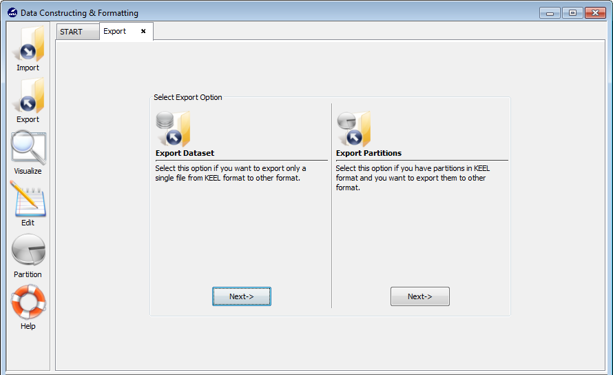
3.2.1 Export dataset
Select this option if you want to export only a single file from KEEL format to other format (see Figure 70).

This option consists of the next parts:
- Step 1. Select the source file. First of all, the path of source file must
be specified as shown in Figure 71 (a browser commonly known from
many other GUI programs is used to define this path).
- Step 2. Select Input Format. After choosing the file, you must select the
format of destination file. The formats admitted are CVS, TXT, PRN, C4.5,
Excel, DIF, PropertyList and Weka. The different options are shown in
Figure 72.
The Options button allows you to configure, if necessary, a certain separator and null value used in the source file (Figure 73).
Step 3. Save the files. Once the type of conversion and path of file has been configured, you must click on the Next button and then, the original and the exported file are shown (see Figure 74).
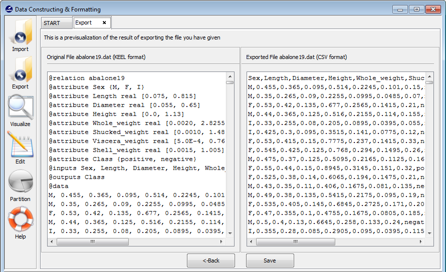
If we agree with the conversion done, click on the Save button and you can select the destination directory for the transformed dataset.
3.2.2 Export partitions
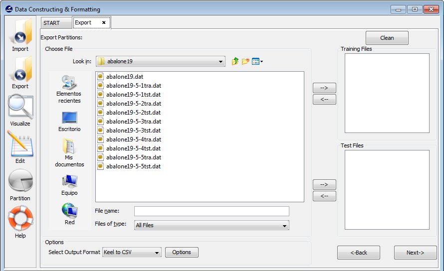
Select this option if you have previously performed partitions in KEEL format and you want to export them to other format. This option allows the selection of a set of training and test files separately. Figure 75 shows the window with that features this option.
This option consists of the following parts:
- Step 1. Select the source files. First of all, the path of source file must be specified. Arrows need to be used for including the files properly in the -training or test sets (as shown in Figure 71).
- Step 2. Select Input Format. After choosing the file, you must select
the type of conversion. The formats admitted are CVS, TXT, PRN,
C4.5, Excel, DIF, PropertyList and Weka. The different options were
shown in Figure 72.
As in the case of the full dataset, the Options button allows you to configure if it is necessary a certain separator and null value used in the source file (Figure 73).
- Step 3. Save the files. Once the type of conversion and path of file
have been configured, you must click Next button and the original
and the exported file are shown (see Figure 74).
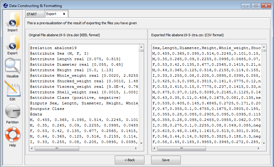
If you agree with the conversion done, click on the Save button and select the destination directory for the transformed dataset.
3.3 File formats
There are different formats of data that can be used to work with the KEEL software suite. In the following, we will show the different available formats that can be used to import/export data. The last format that will be described is the KEEL format that is the one used within the KEEL experiments.
3.3.1 CVS data file format
The CSV file (comma-separated-values) is one implementation of a delimited text file, which uses a “comma”’ to separate values. The CSV file format is very simple and is supported by almost all spreadsheets and database management systems.
The characteristics associated to the CVS file format are the following:
- The first record in a CSV file may be a header record containing name of the columns.
- Each record in a file can have less fields that the number of header columns. In this case, empty values are considered missing values.
- Each row must have the same number of fields separated by commas.
- Two adjacent commas or comma at the beginning or end of the line (space-characters) indicates null values.
- Leading and trailing space-characters adjacent to comma field separators are ignored.
- Each record is one line terminated by a newline character or a carriage return.
- Blank lines will be ignored.
- Fields that contain double quote characters must be surrounded by double quotes, and each one of the embedded double quotes must be represented by a pair of consecutive double quotes.
- Fields with leading or trailing spaces or commas must be delimited with double quote characters.
- The delimiter character can be another one different to comma. Many implementations of CSV allow an alternate separator to be used, such as a tab character and the resulting format is called TSV (Tab Separated Values).
- The last record in a file can be finished or not with the character end of line.
- These files are stored, by default, with the extension CSV.
A CSV (Comma-Separated Values) data file is usually built following the next file format:
value11, value12, ..., value1N
...
valueM1, valueM2, ..., valueMN
An example of a valid CSV file is:
Johnathan,Doe,”ABC Company”,”johndoe@abccompany.com”
Harrie,Wong,”Company Inc.”,”hwong@myprovider.com”
Mary,”Jo Smith”,”Any Corp.”,”mjsmith@myprovider.com”
In the following example we can see the use of some of the rules explained before, such as, the null value expressed in two consecutive commas and the use of double quotes to use the comma character as part of the data and not as a separator.
”1960:1”,14.2,362,,270.7
”1960:2”,14.1,365.9,,273.4
”1960:3”,14.6,367.6,,273.9
”1960:4”,13.2,369.2,,273.3
”1961:1”,10.8,72.9,,273.7
”1961:2”,11.7,378.4,,277.6
”1961:3”,12.2,385.1,,282.2
”1961:4”,13.7,393.2,,288.4
3.3.2 TXT and TVS data file format
A TXT (Text Separated by Tabs) or TSV (Tab Separated Values) file, is a simple text data that allows tabular data to be exchanged between applications with a different internal format. Values separated by tabs have been officially registered as a MIME type (Multipurpose Internet Mail Extensions) under the name text/tab-separated-values.
The characteristics associated to the TXT or TVS file format are the following:
- A file in TXT format consists of lines. Each line contains fields separated from one another by the tab character (horizontal tab, HT, code control 9 in ASCII).
- Fields can be any string of characters, excluding tabs. However, tabs usually don’t appear in data items that you wish to tabulate, so this is seldom a restriction. There are various other formats which are very similar to TSV but use a different separator, such as Comma Separated Values (CSV) which uses the comma as separator. Commas, spaces, and other characters often used as separators in such formats appear rather often in data to be tabulated, at least in header fields.
- Each line must contain the same number of fields.
- The first line contains the name of the fields or attributes, i.e. the column headers.
- An empty value is displayed as an empty field between tabs.
- Such files can be read and edited by any text editor.
- Although TSV is a text format, this type of format is not expected to have a nice tabular visualization when it is printed with an editor or shown on the screen.
- The extension for this type of file is TXT or TSV.
A TXT (Text Separated by Tabulators) or TSV (Tab/Text Separated Values) data file is usually built following the next file format:
value11<TAB> value12<TAB> ... <TAB> value1N
...
valueM1<TAB> valueM2<TAB> ... <TAB> valueMN
An example of valid TXT or TSV file is:
Johnathan <TAB> Doe <TAB> ABC Company <TAB> johndoe@abccompany.com
Harrie <TAB>Wong <TAB> Company <TAB> Inc. hwong@myprovider.com
Mary <TAB> Jo Smith <TAB> Any <TAB> Corp <TAB> mjsmith@myprovider.com”
3.3.3 PRN data file format
This format has the same features and restrictions than the CSV format. The main difference is the separator between fields in the PRN format, which are spaces. However, the spaces in the PRN format have a different role than in CSV files.
The characteristics associated to the PRN file format are the following:
- The first record in a PRN file may be a header record containing the name of the columns.
- Each record in a file with headers in columns can have fewer fields than the number of headers. In this case, empty values are considered missing values.
- Each row must have the same number of fields separated by spaces.
- Several spaces together will be treated as a single space.
- The spaces at the beginning or end of the line indicate null values.
- Each record is one line terminated by a newline character or a carriage return.
- The blank lines will be ignored.
- The fields can contain double quotes, carriage returns (or any other character).
- Fields that contain space characters as values must be surrounded by double quotes.
- The last record in a file does not need to end with the end of line symbol.
- These files are stored by default with the extension PRN.
PRN files have the data separated by blank spaces. A PRN data file is usually built following the next file format shown in Figure 82:
An example of a valid PRN file is (Figure 83):
1 26.99 48.5 22.92
2 26 49.93 20.83
3 26.24 49.96 20.13
4 25.76 49.48 19.98
5 26.73 49.43 19.74
6 24.93 49.83 18.86
7 25.84 49.01 18.23
8 25.91 49.73 17.79
9 24.6 50.15 17.1
3.3.4 DIF data file format
A DIF file (Data Interchange Format) is a text file that is used to import/export between different spreadsheet programs such as Excel, StarCalc, dBase, and so on. This type of format is stored with the extension DIF.
The characteristics associated to the DIF file format are the following:
- The format consists of a header followed by a data block. The header
starts with a file with ASCII text format (Figure 84), where.
- string is any string, it is often the filename or another information.
- columns is the number of columns of an Excel spreadsheet by means of name.
- rows indicates the number of rows of an Excel spreadsheet by means of name.
- The header ends with the following information (Figure 85):
This header is followed by the cells and records of the spreadsheet with the information.
- The structure of the data record has the following format:
where data-type admits various types: SPECIAL, NUMERIC, and STRING, represented by -1, 0 and 1 respectively.
- SPECIAL type
BOT and EOD are strings without quotation marks. BOT represents the start of the table and EOD the end of data section.
- NUMERIC type
value-indicator indicates the data type stored in data:
- TRUE: 1.
- FALSE: 0.
- V: any numerical value.
- NA: missing value.
- ERROR: 0.
- STRING type
string is any text characters.
- SPECIAL type
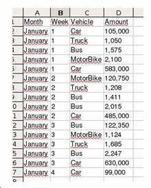
An example of a valid DIF file is:
| Month | Week | Vehicle | Quantity |
| January | 1 | Auto | 105.000 |
| January | 1 | Lorry | 1.050 |
| January | 1 | Bus | 1.575 |
The internal format of a DIF file generated is the following:
0,1 ”Vehicle” V
”EXCEL” 1,0 1,0
VECTORS ”Quantity” ”Lorry”
0,4 -1,0 0,1.050
”” BOT V
TUPLES 1,0 -1,0
0,4 ”January” BOT
”” 0,1 1,0
DATA V ”January”
0,0 1,0 0,1
”” ”Auto” ”Bus”
-1,0 0,105.000 0,1.575
BOT V V
1,0 -1,0 -1,0
”Month” BOT EOD
1,0 1,0
”Week” ”January”
3.3.5 C4.5 data file format
Data files can also be encoded according to the C4.5 format. This format consists of two files, one of them is a name file with the extension NAMES, the other one is a data file with the extension DATA.
The characteristics associated to the NAMES file are the following:
- The NAMES file contains a series of entries that describe the classes, attributes and values of the dataset. Each record is terminated with a point, but the point can be omitted if it would have been the last character on a line). Each name consists of a string of characters without commas, quotes or colons (unless escaped by a vertical bar, |).
- A name can contain a point, but this point must be followed by a white space.
- Embedded white spaces are permitted but multiple white spaces are replaced by a single space.
- The first record in the file lists the names of the classes, separated by
commas and terminated by a point. Each successive line then defines
an attribute, in the order in which they will appear in the DATA files,
with the following format:
<attribute-name: attribute-type>.
The attribute-name is an identifier followed by a colon. The attribute type which must be one of the following values:
- continuous: if the attribute has a continuous values.
- discrete <n>: the word ‘discrete’ followed by an integer which indicates how many values the attribute can take.
- ignore: indicates that this attribute should be ignored.
- A | (vertical bar) means that the remainder of the line should be considered as a comment.
- These files are stored, by default, with the extension NAMES.
A NAMES file is usually built following the next file format:
characteristic-1: domain.
characteristic-2: domain.
...
characteristic-M: domain.
The characteristics associated to the DATA file are the following:
- The file contains one line per object. Each line contains the values of the attributes sorted according to the NAMES file, followed by the class of the object, with all entries separated by commas.
- The format is same than a CVS file (comma separated values), as explained in the CVS data file format.
- Missing values are indicated by ‘?’.
- These files are stored, by default, with the extension DATA.
A DATA file is usually built following the next file format:
An example of a valid C4.5 data file is:
- Content of the NAMES file:
| Firstly the name of classes
good, bad.
| Then the attributes
dur: continuous.
wage1: continuous.
wage2: continuous.
wage3: continuous.
cola: tc, none, tcf.
hours: continuous.
pension: empl contr, ret allw, none.
stby_pay: continuous.
shift_diff: continuous.
educ_allw: yes, no.
holidays: continuous.
vacation: average, generous, below average.
lngtrm_disabil: yes, no.
dntl_ins: half, none, full.
bereavement: yes, no.
empl_hplan: half, full, none.
Figure 93: Example of a C4.5 NAMES file
- Content of the ’.data’ file:
2,5.0,4.0,?,none,37,?,?,5,no,11,below average,yes,full,yes,full,good
3,2.0,2.5,?,?,35,none,?,?,?,10,average,?,?,yes,full,bad
3,4.5,4.5,5.0,none,40,?,?,?,no,11,average,?,half,?,?,good
3,3.0,2.0,2.5,tc,40,none,?,5,no,10,below average,yes,half,yes,full,bad
Figure 94: Example of a C4.5 DATA file
3.3.6 Excel data file format
Microsoft Excel is a spreadsheet program written and distributed by Microsoft. It is currently one of the most widely used spreadsheet suites for operating systems like Microsoft Windows and Apple OS X. Microsoft Excel is integrated as part of the Microsoft Office office suite.
A spreadsheet is a program that allows you to manipulate numerical and alphanumeric data. Spreadsheets are arranged in rows and columns. The intersection of a row/column is called cell.
Each cell can contain data or a formula that can refer to the contents of other cells. A spreadsheet contains 256 columns, which are labeled with letters (from A to IV) and the rows with numbers (from 1 to 65,536), making a total of 16,777,216 cells by spreadsheet.
Because of the versatility of modern spreadsheets, they are used to sometimes to make smaller databases, reports, and other uses. The Microsoft Excel format has the XLS extension.
An example of a valid Excel file is:
3.3.7 Weka data file format
Weka (Waikato Environment for Knowledge Analysis) is a suite of machine learning software written in Java, developed at the University of Waikato, New Zealand. Weka is free software available under the GNU General Public License. It is also a popular software for machine learning and data analysis. Its files are stored by default with the extension ARFF.
The characteristics associated to the ARFF file format are the following:
- Headline. The relation name is defined as the first line in the ARFF
file. The format is: @relation <relation-name>
where <relation-name> is a string. The string must be quoted if the name includes spaces.
- Declaration of attributes. Attribute declarations take the form of an
ordered sequence of @attribute statements. Each attribute in the
dataset has its own @attribute statement which uniquely defines
the name of that attribute and its data type. The order in which
the attributes are declared indicates the column position in the data
section of the file. For example, if an attribute is declared in the third
position then, Weka expects that all values related to that attribute
will be placed in the third column delimited by commas. The format
for the @attribute statement is:
@attribute <attribute-name> <datatype>
<attribute-name>: must start with an alphabetic character. If spaces are to be included in the name then the entire name must be quoted.
<datatype>: can be any of the four types supported by Weka version 3.2.1:
- NUMERIC or REAL. Numeric attributes can be real numbers.
- INTEGER. Integer attributes can be integer numbers.
- DATE. Date attributes are an optional string specifying how date values should be parsed and printed. The default format string accepts the ISO-8601 combined date and time format: “yyyy-MM-dd’T’HH:mm:ss”.
- STRING. String attributes allow us to create attributes containing arbitrary textual values.
- ENUMERATE. Enumerate attributes consist of a set of possible
values separated by commas (characters or strings), which define
the values that can be used for the specified attribute. For
example, if we have an attribute that indicates the time might be
as:
@attribute time sunny, rainy, cloudy
- Section data. The data section of the file contains the data declaration line
and the actual instance lines. The @data declaration is a single line
denoting the start of the data segment in the file. The format is:
Each instance is represented on a single line, with carriage returns denoting the end of the instance.
Attribute values for each instance are delimited by commas. They must appear in the order that they were declared in the header section (i.e. the data corresponding to the n-th @attribute declaration is always the n-th field of the attribute).
Missing values are represented by a single question mark, as in:
Some additional specifications of the ARFF format are:
- The relationship and attributes names are stored in a string type. This string type is the same data type than the string type used on Java.
- If any name contains spaces it is necessary to include double quotes.
- If you need to indicate a missing value, you have to use symbol ‘?’.
- The separation symbol for data in @data section is a comma.
- A % symbol means that the remainder of the line should be considered as a comment.
- These files are stores, by default, with the extension ARFF.
A Weka data file is usually built following the next file format shown in Figure 98:
@attribute <attribute-name-1> <datatype>
...
@attribute <attribute-name-N> <datatype>
@data
value11,value12,value1N
...
valueM1,valueM2,valueMN
An example of a valid Weka file is shown in Figure 99:
@relation weather
@attribute outlook sunny, overcast, rainy
@attribute temperature real
@attribute humidity real
@attribute windy TRUE, FALSE
@attribute play yes, no
@data
sunny,85,85,FALSE,no
sunny,80,90,TRUE,no
overcast,83,86,FALSE,yes
rainy,70,96,FALSE,yes
rainy,68,80,FALSE,yes
3.3.8 XML data file format
XML (EXtensible Markup Language) is a set of rules to define semantic labels that organize a document in different parts. XML is a meta-language that defines the syntax to define other structured label languages.
Not all XML files describe data files. In the following, the basic features of the XML format will be defined, with an special interest in how these files are built to storage data:
- The first line must follow the next structure:
?Xml version=”1.0” encoding=”UTF-8” standalone=”yes”
This line can feature some options for the XML file. Some of them are mandatory while others are entirely optional:
- version: indicates the XML version used in the document. This field is compulsory.
- encoding: indicates how the document is encoded. The default option is using UTF-8, but other options can also be used, such as UTF-16, US-ASCII, ISO-8859-1 and so on. This field is optional.
- standalone: specifies whether further documents, such as a DTD, are required to process the document. The default value is ”no”.
- XML documents must follow a hierarchical structure by means of labels. XML elements can contain other elements. Elements may also have attributes; these are always expressed as name-value pairs in the element’s open tag.
- A well-formed document must follow the next rules:
- Element names are case sensitive, that is, the following is a well-formed matching pair <step>…</step>, whereas this is not <step>…<step>.
- Non-empty elements are delimited by both a start-tag and an end-tag.
- Attribute values must always be quoted, using single or double quotes, and each attribute name should appear only once in any element.
- All spaces and carriage returns are taken into account in the elements.
- The element names should not begin with the letters “xml”.
- The element names should not use character “:”.
- Although it is permissible to use the characters “.” and “-” in element names, it is not recommended because the application which processes XML files may interpret these signs as operators. Therefore, these characters will be replaced in KEEL by the character “_”.
- The character ”\” should not be used in the names of elements.
- The names may contain any alphanumeric character, but they cannot start with a numerical or punctuation character.
- Special characters can be represented either using entity references, or by
means of numeric character references. An example of a numeric character
reference is “€”, which refers to the Euro symbol using its Unicode
codepoint in Hexadecimal.
An entity reference is a placeholder that represents that entity. It consists of the entity’s name preceded by an ampersand (“&”) and followed by a Semicolon (“;”). XML has five predeclared entities:
- & (ampersand) &
- < (less than) <
- > (greater than) >
- ’ (apostrophe) '
- ” (quotation mark) "
- Comments can be placed anywhere in the tree, including text, if the content
of the element is text. XML comments start with <!- and end with
->.
<!- This is a comment ->
- XML requires that elements be properly nested, that is, elements may never
overlap. For example, the code below is not well-formed XML, because the
<em> and <strong> elements overlap:
<!-- WRONG! Not well-formed XML! -->
<p>Normal
<em>emphasized
<strong>strong emphasized</em>
strong</strong>
</p> - All XML documents must contain a single tag pair to define the root element. All other elements must be nested within the root element. All elements can have sub (children) elements. Sub elements must be in pairs and correctly nested within their parent element.
- The <root> label indicates the start point of the data. This label can have any name. If any children of the <root> label does not have the same name on the <row> label, the user must enter the name of this tag, otherwise it is assumed that all children have the same value.
- Each <row> label is the parent of nAtts labels, where nAtts is the number of attributes that are available in the data. The name of each of these children labels will be the attribute name, and the value associated to the label is the data value of the attribute.
- There are as many <row> labels as the available rows of data.
A XML data file for the KEEL suite is usually built following the next file format (Figure 100):
<root>
<row1>
<att-name-1>att-value-11</att-name-1>
<att-name-2>att-value-12</att-name-2>
<att-name-N>att-value-1N</att-name-N>
</row1>
...
<rowM>
<att-name-1>att-value-M1</att-name-1>
<att-name-2>att-value-M2</att-name-2>
<att-name-N>att-value-MN</att-name-N>
</rowM>
</root>
Another XML data file format valid for the KEEL suite is shown in Figure 101
<root>
<row1>
<field name=”att-name-1”>att-value-11</field>
<field name=”att-name-2”>att-value-12</field>
<field name=”att-name-N”>att-value-1N</field>
</row1>
...
<rowM>
<field name=”att-name-1”>att-value-M1</field>
<field name=”att-name-2”>att-value-M2</field>
<field name=”att-name-N”>att-value-MN</field>
</rowM>
</root>
An example of a valid XML is depicted in Figure 102
<root>
<customer>
<id>5</id>
<course>66</course>
<name>My book</name>
<summary>Book summary</summary>
<numbering>2</numbering>
<disableprinting>0</disableprinting>
<customtitles>1</customtitles>
<timecreated>1114095924</timecreated>
<timemodified>1114097355</timemodified>
</customer>
<customer>
<id>6</id>
<course>207</course>
<name>My book</name>
<summary>A test summary</summary>
<numbering>1</numbering>
<disableprinting>0</disableprinting>
<customtitles>0</customtitles>
<timecreated>1114095966</timecreated>
<timemodified>1114095966</timemodified>
</customer>
</root>
In this example there are:
- 9 attributes, named id, course, name, summary, numbering, disableprintg, customtitles, timecreated and timemodified.
- 2 instances with these 9 attributes.
- The main label is <root>.
- The label <customer> contains each instance. If this XML data file is imported/exported to the KEEL software suite, the name of this label will be the same than the name of data relation stored in the KEEL format.
The following example (Figure 103) presents another XML data structure, but contains the same data than the previous example.
<root>
<row>
<field name=”id”>5</field>
<field name=”course”>66</field>
<field name=”name”>My book</field>
<field name=”summary”>Book summary</field>
<field name=”numbering”>2</field>
<field name=”disableprinting”>0</field>
<field name=”customtitles”>1</field>
<field name=”timecreated”>1114095924</field>
<field name=”timemodified”>1114097355</field>
</row>
<row>
<field name=”id”>6</field>
<field name=”course”>207</field>
<field name=”name”>My book</field>
<field name=”summary”>A test summary</field>
<field name=”numbering”>1</field>
<field name=”disableprinting”>0</field>
<field name=”customtitles”>0</field>
<field name=”timecreated”>1114095966</field>
<field name=”timemodified”>1114095966</field>
</row>
</root>
3.3.9 HTML data file format
HTML, an extension of Hypertext Markup Language, is the predominant markup language for web pages. It provides a means to describe the structure of text-based information in a document (denoting certain text as headings, paragraphs, lists, and so on) and to supplement that text with interactive forms, embedded images, and other objects. HTML is written in the form of labels (known as tags), surrounded by angle brackets.
HTML is an application of SGML according to the international standard ISO 8879. XHTML is a reformulation of HTML 4 as an XML application 1.0, and allows compatibility with user agents already admitted HTML 4 following a set of rules.
The basic HTML tags are:
- <HTML>: is the label that defines the beginning of the document.
- <HEAD>: defines the header of the document. This header normally
contains information about the page such as the title, meta tags for
proper search engine indexing, style tags, which determines the page
layout and JavaScript coding for special effects. Within the header
<HEAD> we find:
- <TITLE>: defines the title of the page. This will be visible in the title bar of the browser.
- <LINK>: defines some advanced features, for example style sheets used for the design of the page.
- <BODY>: contains the main content of the page, this is where the content of
the document begins and where the html codes will be placed. It defines
common properties to the entire page, such as the background color and
margins. Within the body a great variety labels can be used. The labels
which are interesting for the KEEL software suite are the ones related to
tables in HTML:
- <TABLE>: This label defines the beginning of a table (<TR> represents rows and <TD> represents cells).
A HTML file is usually built following the previously described format, which is shown in Figure 104:
The HTML table model enables the arrangement of data like text, preformatted text, images, links, forms, form fields, other tables, and so on, into rows and columns of cells.
Tables are defined with the <TABLE> tag. A table is divided into rows (with the <TR> tag), and each row is divided into data cells (with the <TD> tag). The tag TD stands for table data which is the content of a data cell. A data cell can contain text, images, lists, paragraphs, forms, horizontal rules, tables, etc.
The different tags which will define the structure of the table for obtaining a valid data file are:
- TR: The label <TR> allows to insert rows in the table.
- TH: The label <TH> allows to define the head table.
- TD: The label <TD> allows to insert cells in each row. Any element can be inserted in it, like pictures, lists, formatted text and even other tables.
An HTML data file valid for KEEL is usually built following the next file format (Figure 105:
<tr>
<th>Header 1</th>
<th>Header 2</th>
<th>Header 3</th>
</tr>
<tr>
<td>Value 1</td>
<td>Value 2</td>
<td>Value 3</td>
</tr>
<tr>
<td>Value 4</td>
<td>Value 5</td>
<td>Value 6</td>
</tr>
</table>
An example of a valid HTML file is the following (Figure 106):
<head>
<h1 align=”center”>VEHICLES</h1>
</head>
<body>
<table border=”1” cellspacing=”1” cellpadding=”0”>
<tr align=”center”>
<td>Month</td>
<td>Week</td>
<td>Vehicle</td>
<td>Amount</td>
</tr>
<tr>
<td>January</td>
<td>1</td>
<td>Car</td>
<td>105.0</td>
</tr>
<tr>
<td>January</td>
<td>1</td>
<td>Truck</td>
<td>1.05</td>
</tr>
<tr>
<td>January</td>
<td>1</td>
<td>MotorBike</td>
<td>1.575</td>
</tr>
</table>
</body>
</html>
3.3.10 KEEL data file format
All the other data formats described in this section can be imported/exported to the KEEL data file format. This format is used in KEEL experiments and associated operations. KEEL data files are represented as plain ASCII text files, named with the DAT extension.
Each KEEL data file is composed by 2 sections:
- Header: Basic metadata describing the dataset.
- Data: Content of the dataset.
Comments are allowed in both sections using the “%” character.
The header is composed by the following metadata:
- @relation: The name of the dataset.
- @attribute: Describes one attribute of the data (a column). It is
possible to define three different types of attributes:
- integer: @attribute <name> integer
 min, max
![]](Principal1x.png)
- real: @attribute <name> real
 min, max
![]](Principal3x.png)
- nominal: @attribute <name>
 Value1,value2,…,valueN
The <name> is the identifier of the attribute. Its maximum length is 12 characters. The min and max values for integer and real attributes, and the list of possible values for nominal attributes, are optional. If they are missing, the corresponding values will be extracted from the data by the KEEL software suite.
- integer: @attribute <name> integer
- @inputs: Identifiers of the attributes which will be processed as inputs.
- @outputs: Identifiers of the attributes which will be processed as outputs.
The @inputs and @outputs definitions are optional. If they are missing, all the attributes will be considered as input attributes, except the last, which will be considered as the output attribute.
@attribute mcv nominal {a,b,c}
@attribute alkphos integer [23, 138]
@attribute sgpt integer [4, 155]
@attribute sgot integer [5, 82]
@attribute gammagt integer [5, 297]
@attribute drinks real [0.0, 20.0]
@attribute selector {true,false}
@inputs mcv, alkphos, sgpt, sgot, gammagt, drinks
@outputs selector
The data instances are represented as rows of comma separated values, where each value corresponds to one attribute, in the order defined by the header. Missing or null values are represented as <null> or ?.
If the dataset corresponds to a classification problem, the output type must be nominal:
@attribute selector {true,false}
...
@outputs selector
@data
a, 92, 45, 27, 31, 0.0, true
a, 64, 59, 32, 23, <null>, false
b, 54, <null>, 16, 54, 0.0, false
If the dataset corresponds to a regression problem, the output type must be real:
@attribute selector real [0.0, 20.0]
...
@outputs selector
@data
a, 92, 45, 27, 31, 0.0, 0.9
a, 64, 59, 32, 23, <null>, 17.5
b, 54, <null>, 16, 54, 0.0, 3.5
A full example of a valid KEEL file is shown in Figure 110:
@relation bupa2
@attribute mcv nominal {a,b,c}
@attribute alkphos integer [23, 138]
@attribute sgpt integer [4, 155]
@attribute sgot integer [5, 82]
@attribute gammagt integer [5, 297]
@attribute drinks real [0.0, 20.0]
@attribute selector {true,false}
@inputs mcv, alkphos, sgpt, sgot, gammagt, drinks
@outputs selector
@data
a, 92, 45, 27, 31, 0.0, true
a, 64, 59, 32, 23, <null>, false
b, 54, <null>, 16, 54, 0.0, false
a, 78, 34, 24, 36, 0.0, false
a, 55, 13, 17, 17, 0.0, false
b, 62, 20, 17, 9, 0.5, true
c, 67, 21, 11, 11, 0.5, true
a, 54, 22, 20, 7, 0.5, true
3.4 Visualize data
The visualization options provide graphical information about existing KEEL datasets. There are different options related to this graphical information, where an user can select to view the content of a dataset, specific information about the attributes or to compare two attributes using charts.
Figure 111 shows the main window of the visualization menu. First of all, an user must select the path of source dataset (in KEEL format) that is going to be visualized (see Figure 112). When the file is loaded, different information about the dataset is shown according to the option selected.
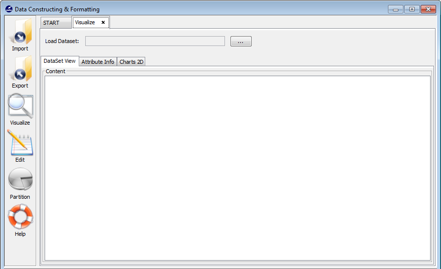

3.4.1 Dataset view
If an user selects to visualize the dataset information, the content of dataset selected will be shown in plain text form. The data cannot be modified; the user can only visualize it (see Figure 113).
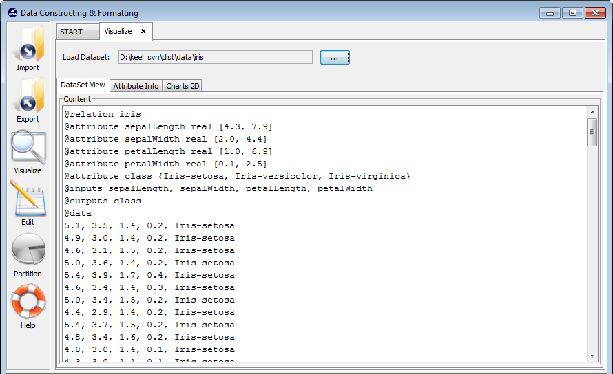
3.4.2 Attribute info
In this option, an user can obtain detailed information about the attributes defined in the dataset. The information showed is the attribute’s type (either integer, real or nominal) and whether the attribute is input or output. Below the attribute information, there are two additional areas that provide further information about the selected attribute within the attribute list.
On the left side, textual information about the attribute will be shown. This information depends on the attribute type. If the attribute is integer or real, then, the rank values, average and variance associated to the data are shown. In the case of a nominal attribute, only its possible values are displayed.
On the right side, graphical information about the selected attribute is provided. Specifically, the distribution of the attribute’s values is shown through a chart. Figure 114 shows how this information is organized for a real attribute and Figure 115 shows which information is provided for a nominal attribute.
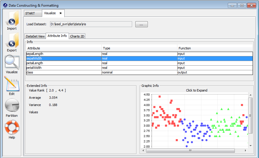
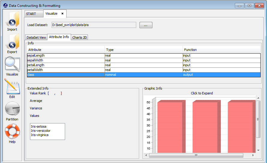
3.4.3 Charts 2D
This option enables an user to contrast a pair of different attributes. In order to do so, an user has to select the two attributes that are going to be compared. There are two drop lists to select the two attributes that are going to be contrasted: each one of these lists contain all attribute of dataset (see Figure 116).
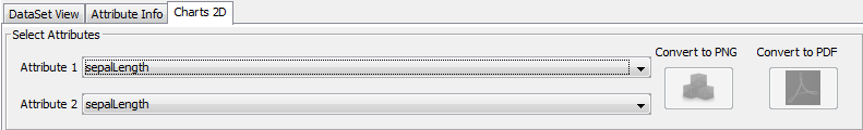
When the attributes are selected, an user has to click on the View chart button and then, a graphic depicting the values of these attributes is shown (Figure 117).
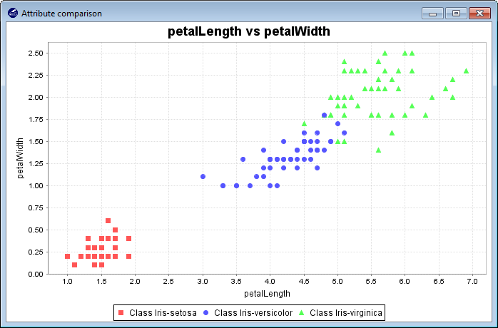
If the generated chart is expected to be introduced in other document, an user should use the buttons: Convert to PNG: this option saves the graph as a PNG image, and Convert to PDF: this option saves the chart as a PDF document (Figure 118).
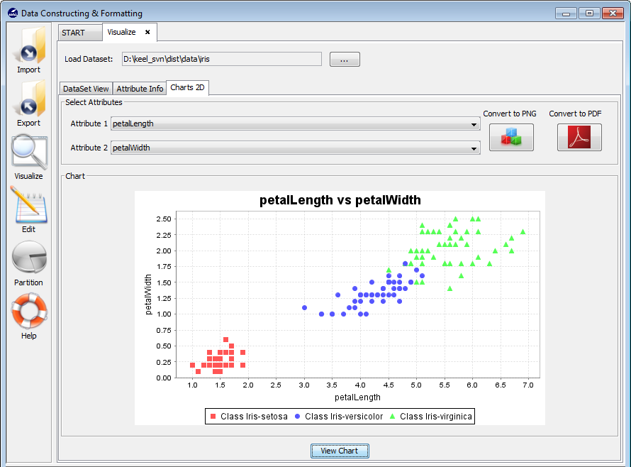
3.5 Edit data
The edit data feature allows an user to edit any existing KEEL datasets in order to add new attributes, to delete others, to correct some errors within the data, and so on.
Figure 119 shows the main window of the edit menu. First of all, an user must select the path of source dataset (in KEEL format) that is going to be edited (see Figure 120).
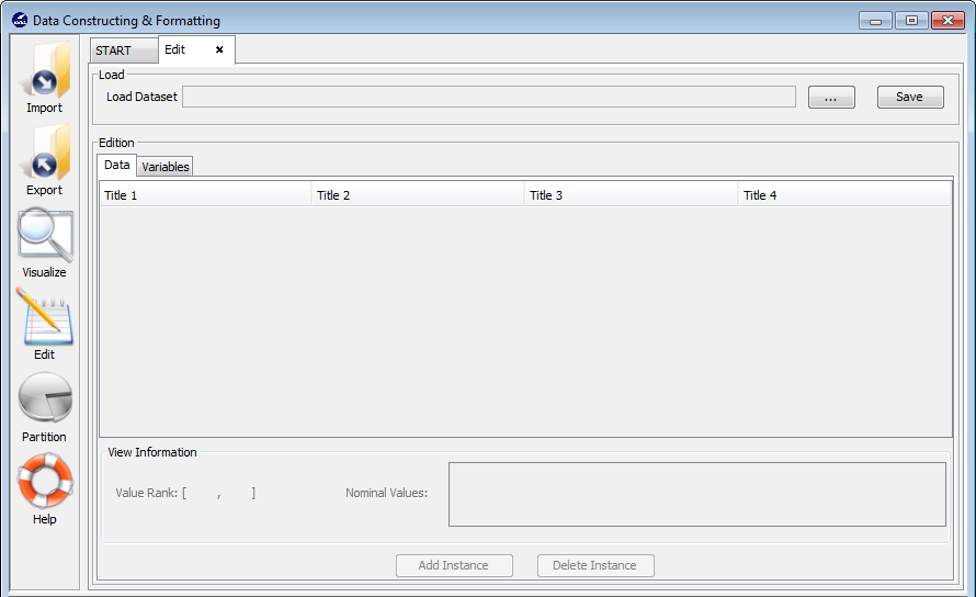
When the file is loaded, its content appears bellow the Load Dataset option, organized in a table, in a Data area. The modifications over this dataset can be performed both over the instances and over the variables. In the following, we will address how an user can alter the values in a dataset from both approaches.
3.5.1 Data edition
This option enables an user to add new instances, delete existing instances or modify any of the available instances in the data (see Figure 121).
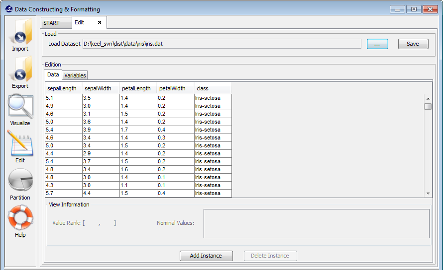
In order to do so, an user has to interact with the table that displays the dataset information and with its associated buttons. The operations that can be performed are:
- Modify the cell content: An user that wants to modify the cell content has to click on the cell that wants to change. Then, the user has to write the new value, and if it is valid, the cell content is modified. Otherwise an error dialog is shown.
- Delete an instance: An user that wants to delete an instance has to click on any of the cells that are associated with the instance (row) that an user wants to delete. Then, a Delete Instance button is activated. When an user clicks on it, the full instance will be deleted.
- Add a new instance: An user that wants to add a new instance has to click on the Add Instance button, which will then add a new instance. If a cell was previously selected, the new instance is added on top of the instance whose cell was selected. If no cell was selected, a new instance is added at the bottom of the table. The new instance will have empty values and the different values can be filled out clicking on the different cells.
3.5.2 Variable edition
In this option different modifications on the variables of the selected dataset can be carried out (see Figure 122).
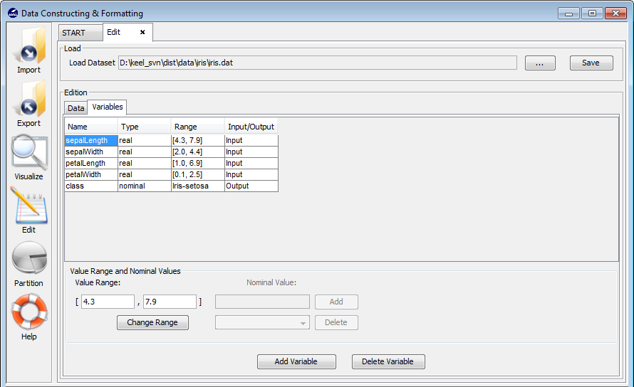
In order to do so, an user has to interact with the table that displays the dataset information and with its associated buttons. The operations that can be performed are:
- Add new variables: An user that wants to add new variables has to click on the Add Variable button. Then, a new row is added at the bottom of the table which can be filled with the values that an user considers appropriate.
- Delete a variable: An user that wants to delete a variable has to first select the variable that is going to be erased and then, click on the Delete Variable button.
- Change the rank values: If an user wants to change the rank values, first of all, this user has to select a real or integer variable. If the variable selected is integer or real, the user can modify its rank values and then click on the Change Range button to change the information.
- Change nominal values: If an user wants to change the nominal values, this user has to select a nominal variable. If the variable selected is nominal, an user can add or remove the values allowed for that variable using the list and the Delete and Add buttons.
- Change attribute type: An user that wants to change the variable type, has to click on the cell that contains the information about the attribute and the type. That is, the cell whose row represents the variable that is going to be changed and the Type column. Then, the user can modify the variable type using the drop-down list that is shown specifying any other type of variable.
- Change attribute function: An user that wants to change the attribute function has to click on the cell that contains the information about the attribute and the function. That is, the cell whose row represents the variable that is going to be changed and the Input/Output column. Then, the user can modify the variable “function” using the drop-down list that is shown specifying if it is an input or output attribute.
When all the changes to data have been applied, an user can save them to a file clicking on the Save button.
3.6 Data partition
The data partition feature enables an user to make partitions from an existing dataset in KEEL format. Figure 123 shows the main window of this option.
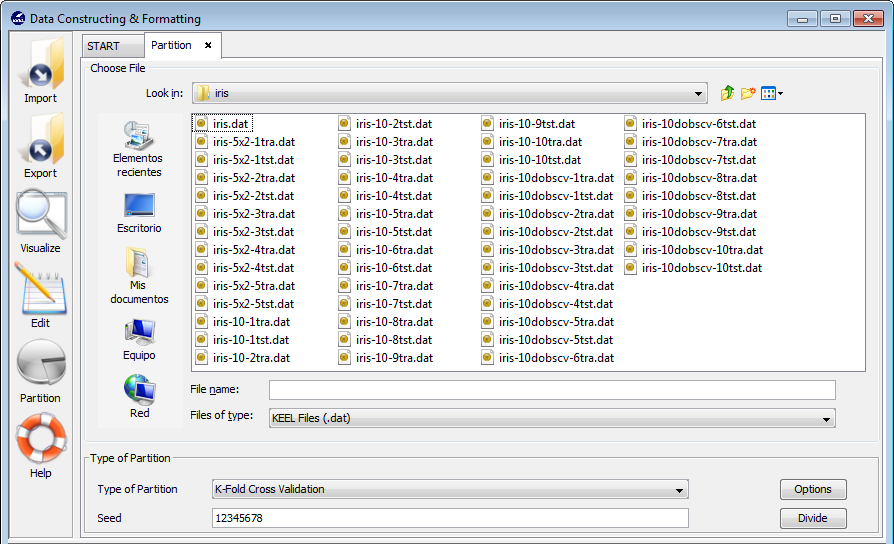
To create partitions from a given dataset, an user has to follow the next steps:
- Step 1. Choose File. First of all, an user must choose the path of the full dataset in KEEL format that is going to be the source for the partitions that are going to be created.
- Step 2. Select Type of Partitioning. Once the file has been selected,
you have to choose the type of partitioning. The available types of
partition are:
- K-fold cross validation: This partitioning technique obtains k random partitions of data, dividing the original data into k parts, where the combination of k- 1 of them is considered as training set and the remaining one is treated as test set. This option allows the user to configure the number of folds (k) of the partitions; to do so, the user has to click on the Options button.
- 5x2 cross validation: This partitioning technique randomly obtains 5 pairs of training and test data. This partitioning technique has no options.
- DOB-SCV: This partitioning technique obtains k partitions of data, dividing the original data into k parts, where the combination of k- 1 of them is considered as training set and the remaining one is treated as test set. The k partitions of data are computed to alleviate the dataset shift problem, placing groups of k nearest examples in different folds. This option allows the user to configure the number of folds (k) of the partitions; to do so, the user has to click on the Options button.
- Step 3.Specify the Seed. To create the partitions of the dataset, it is
necessary to specify the seed for the random generator that will be used
during the partitioning process.
- Step 4. Create the Partitions. When the previous steps have been configured, the partitions will be created when the user clicks on the Divide button. The files generated during the partition process are stored in the directory specified in Step 1. The name of these files is given automatically and it depends on the type of the partition selected.
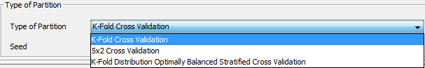

4 Experiment Design
The Experiments Design section goal is to allow an user to create the desired experiments using a graphical interface. To do so, the user is expected to use available datasets and algorithms to generate a file containing a folder structure with all the necessary files needed to run the designed experiments in the processing unit selected by the user.
In this way, an user only needs to select the input data (datasets), the algorithms that want are going to be tested and the connections that define the processing flow that needs to be run. It is possible to concatenate methods, insert statistical tests, and so on. Moreover, the tool allows an easy configuration of the parameters associated to each method: they can be selected using the graphical interface without external configuration files.
This part of KEEL has two main objectives: on the one hand, an user can use the software as a test and evaluation tool during the development of an algorithm. On the other hand, it is also a good option in order to compare new developments with standard algorithms already implemented and available in the KEEL software suite 3.0.
4.1 Configuration of experiments
When the Experiments option is selected, the main window of the Experiments module will appear (Figure 126):
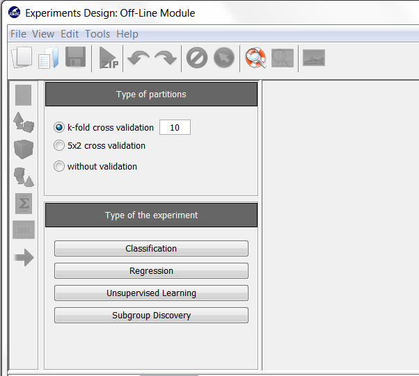
First, it is necessary to select the type of experiment and the type of partitions to employ; the options selected will determine the kind of methods and datasets that will be available to design the experiment.
The types of partitions available (as shown in Figure 127) are the following ones:
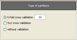
- k-fold cross validation (the value of k must be specified)
- 5x2 cross validation
- without validation
Currently, the KEEL Experiments module offers the following types of experiments:
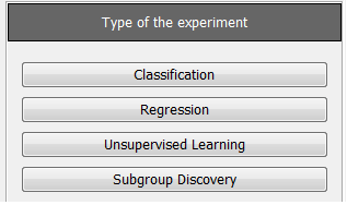
- Classification
- Regression
- Unsupervised Learning
- Subgroup discovery
When the type of experiment has been selected, the datasets selection panel will be shown, allowing continuing the experiment design.
4.2 Selection of datasets
The datasets selection panel shows the available datasets for the current experiment. Its contents will depend of the type of experiment already selected:
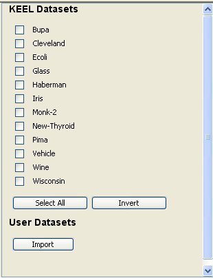
The next step is to choose the wished datasets from the panel. The buttons Select All and Invert allows making the selection easily:

The Import Button allows importing an existing dataset into the KEEL environment, ready to be selected for the current experiment. By clicking on it, the main window of the Data Import Tool will be shown. The process to import a new dataset can is described in the Data Management module section of the manual (Section 3.1).
If a new dataset is added, new buttons will appear allowing the user to Invert the current selection of user datasets, or to Select All of them. Furthermore, it is possible to add even more datasets (with the Import button), or to Remove the datasets selected.
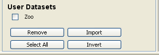
When all the necessary dataset are selected, the experiment design process can continue. To do so, the user must click on the white graph panel to set the datasets node of the experiment.
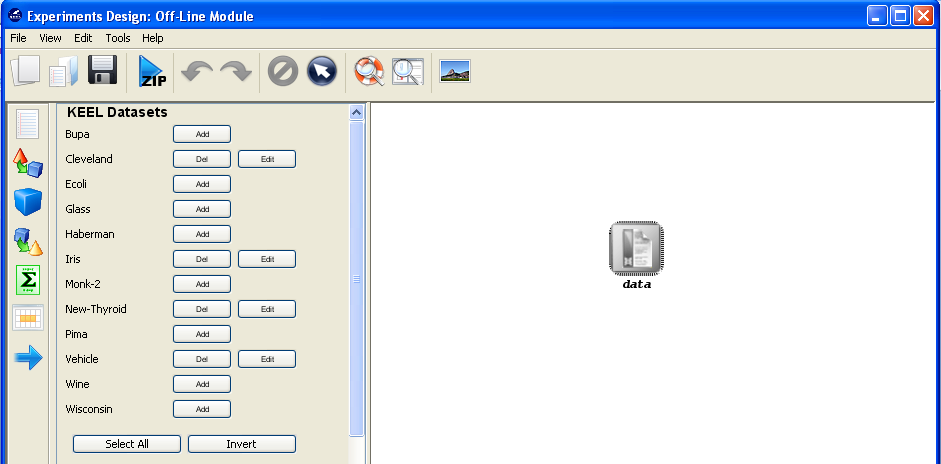
At this point, the KEEL Experiments module will check if all the necessary partitions of the current selected datasets are present. If some missing partitions are found (e.g. if the user selected a k value different from the sets available in the standard distribution), the tool will prompt the following message:
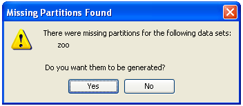
Clicking on yes will result on the generation of the missing partitions inside the KEEL environment. If the user selects to No generate the partitions, this warning will be shown again before the generation of the experiment graph.
4.3 Experiment Graph
The experiment graph shows the components of the current experiment and describes the relationships between them. The user can add new components by using the left menu:
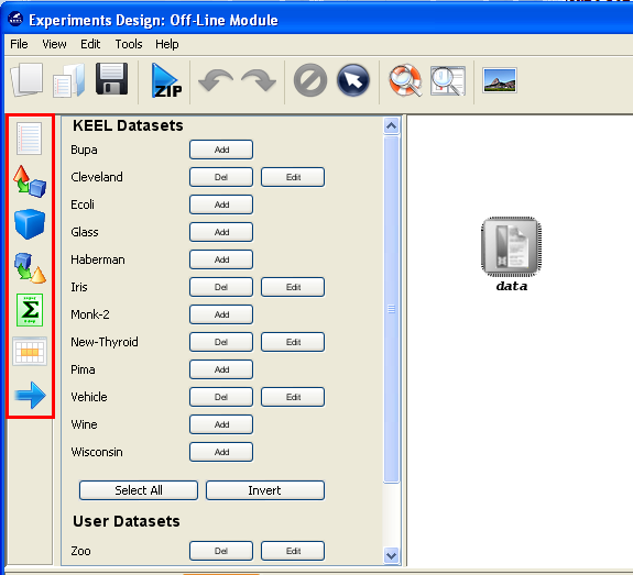
This menu has the following categories available:
 Datasets: Modify the datasets of the experiments.
Preprocessing methods: Preprocess over the initial datasets.
Standard methods: Data mining methods.
 Postprocessing methods: Post-process over the results of standard
methods.
Postprocessing methods: Post-process over the results of standard
methods.
Statistical tests: Statistical procedures to contrast the results achieved in
the experiment.
Visualization modules: Show the results of the experiments in an
upgraded way.
Connections: Links between the components of the experiment.
4.3.1 Datasets
This module lets the user edit the current datasets selected for the
experiment.
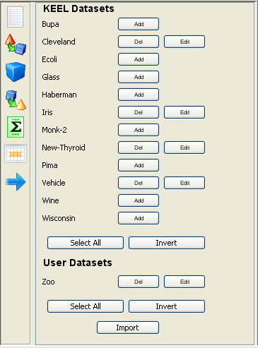
As in the Select Datasets panel, the user can still Add and Delete datasets to the experiment (from those already registered in the KEEL environment). Also, it is still possible to import new datasets.
Furthermore, the button Edit allows the user to indicate which partitions (training and test) desires to use. This way, it is possible to temporally alter the files which will be included in the experiment.
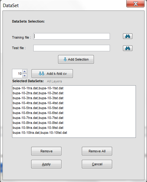
This dialog shows the initial files of the dataset. From it, is possible to Remove a
pair of training a pair of training/test files, to Remove All files. Also, the dialog
allows to Add new pairs of training and test files. To do so, they must be selected
by using the search buttons  :
:
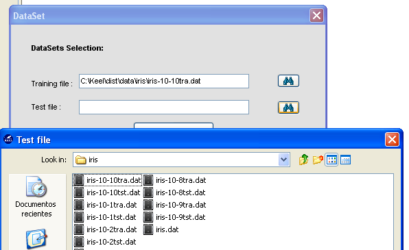
Finally, it is also possible to add a complete set of k-fold cross validation files by selecting the adequate number of folds and pressing the button Add k-fold cv.

4.3.2 Preprocessing methods
This category includes several preprocessing methods
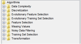
- Data complexity: It can compute twelve different indicators of the source of complexity for the considered dataset.
- Discretization: Methods for converting real or numeric data into nominal data.
- Feature Selection (Standard and evolutionary): Methods to select features of the data.
- Training set Selection (Standard and Evolutionary): Methods to select instances of the data.
- Missing Values: Methods to assess data containing missing values.
- Transformation: Methods for transforming the format of data: Nominal to binary, decimal scaling, and so on.
To add any preprocessing method to the current experiment, it is only needed to select it and click in the graph of the experiment:
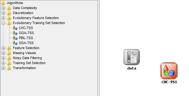
4.3.3 Standard Methods
This category includes the data mining methods included in the KEEL
software suite:
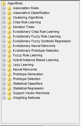
- Association Rules: Methods for extracting association rules from data.
- Associative Classification: Algorithms for mining classification rules following an associative rule mining scheme
- Clustering Algorithms: Clustering methods
- Crisp Rule Learning (Standard and Evolutionary): Interval rule classification algorithms
- Decision Trees: Methods for building decision trees.
- Fuzzy Rule Learning (Standard and Evolutionary): Methods for performing fuzzy rule-based learning.
- Fuzzy Symbolic regression: Methods for performing symbolic regression procedures.
- Hybrid Instance Based Learning: Methods using hyperrectangles (combination of rule induction and instance based learning) to extract knowledge from data.
- Lazy Learning: Learning methods which do not build a model in its training phase.
- Neural networks (Standard and Evolutionary): Artificial neural networks.
- Prototype Generation: Methods for the generation of an optimal training set of prototypes.
- Prototype Selection (Standard and Evolutionary): Methods for reducing the size of the training set without losing precision or accuracy in order to a posterior classification
- Statistical Classifiers: Classifiers based on statistical models.
- Statistical Regression: Construction of statistical models based on data.
- Support Vector Machines: Constructs of a set of hyperplanes in a high-dimensional space for achieving the largest distances among the instances of different classes (the so-called functional margin).
To add any method to the current experiment, it is only needed to select it and click in the graph of the experiment:
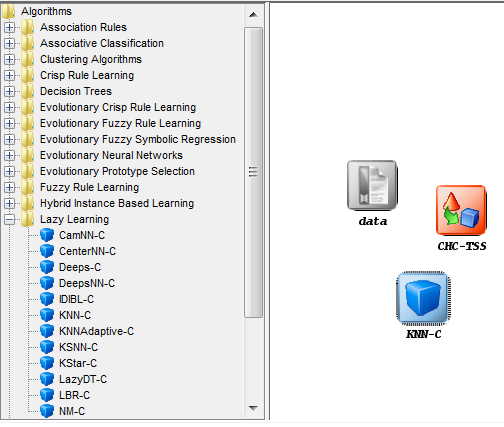
4.3.4 Post-processing methods
This category includes the postprocessing methods included in the KEEL
software suite:
- Fuzzy Rule PostProcessing: Methods for performing a postprocess phase over the results of a Fuzzy Rule extraction method (only for regression tasks).
To add any postprocessing method to the current experiment, it is only needed to select it and click in the graph of the experiment:
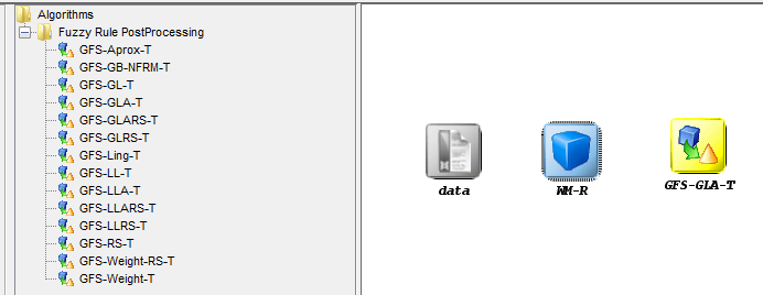
4.3.5 Statistical tests
This category includes several statistical modules available to contrast
experiments performed with the KEEL software suite:
- Tests for Classification: Statistical procedures for contrasting the results of classification experiments.
- Tests for Regression: Statistical procedures for contrasting the results of regression experiments.
To add any statistical procedure to the current experiment, it is only needed to select it and click in the graph of the experiment:
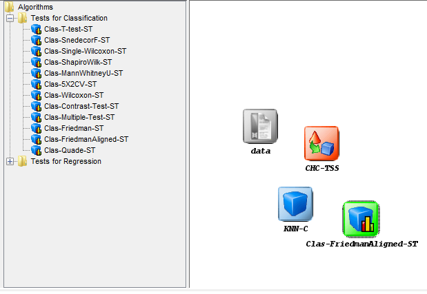
Additionally, a full module is available for carrying out non-parametrical statistical tests of the results obtained by the experiments developed by KEEL or by any other software tool. Please refer to the content of this manual regarding this specific module (Section 7.2).
4.3.6 Visualization modules
This category includes several visualization modules developed to analyze
and summarize the results achieved in the experiments:
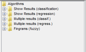
- Show Results (classification): Modules for summarizing results achieved in classification problems.
- Show Results (regression): Modules for summarizing results achieved in regression problems.
- Multiple Results (classification): Modules for analyzing results achieved in classification problems with multiple algorithms.
- Multiple Results (regression): Modules for analyzing results achieved in regression problems with multiple algorithms.
- Fingrams (fuzzy): This module generates the required configuration file to use a stand-alone open source software tool which creates fingrams (http://sourceforge.net/projects/fingrams/)
To add any visualization module to the current experiment, it is only needed to select it and click in the graph of the experiment:
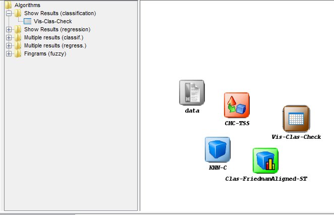
4.3.7 Connections
The connections allow finishing the designing of the experiment, by
connecting the included modules with flows which represent the data flow
in the experiment. They can be used both as inputs or outputs of the
modules.
- Insert connection: to make a connection, select the button from
the left tool bar. Then, click on the source node and finally click on the
target node.
- Restrictions: there are some restrictions that must be considered when
making connections between the different elements:
- A dataset cannot have inputs.
- The pre-processing algorithms can only receive inputs from a dataset or another pre-process method.
- Knowledge extraction methods can receive a flow from a dataset, from a pre-processing algorithm or from a previous method.
- The test and visualization modules must receive input data from a method or from a post-processing algorithm.
- Test and visualization modules cannot have outputs.
- The graph cannot have any cycle.
All these restrictions are verified in execution time when a connection is been created. If one of these connections is not allowed, the application will show an error message. In next figures some examples of incorrect graphs are shown:
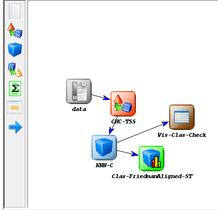
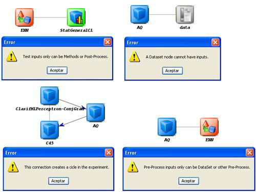
4.4 Graph Management
The graph allows performing the following operations over its elements:
- Parameters configuration menu: it is possible to access to the parameter configuration menu of an algorithm by double clicking with the mouse on a method node in the draw area.
- Objects selection: in order to select a single element, just click with the left button of the mouse over it. But it is possible to select several elements, clicking in an empty zone of the draw area and dragging the mouse until covering all the objects wished.
- Move objects: It is possible to move one or several elements selected with the aid of the left button of the mouse, dragging them to the desired position. Another way is to use the keyboard cursors.
- Remove objects: To remove a module, select it and press Supr key. It is also possible to remove it from the tool bar.
4.5 Algorithm parameters configuration
Once a module has been inserted in the graph, it is possible to configure the value of its parameters. To do so, the user have to double click on the algorithm symbol and a dialog will be shown (Figure 151).

At the top of this dialog it is possible to set the number of times that the algorithm will be executed (only available for random methods). Each execution will be made using a seed generated from the initial seed. The second list allows specifying in which datasets the parameters will be changed.
In the table located in the center of the window, all the algorithm parameters are established to its initial values. These values can be modified, as far as the new values will be appropriate for the specific method; otherwise, an error message will appear, as shown in Figure 152
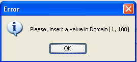
Finally, the Default Values button allows returning all parameter to its default values.
4.6 Generation of Experiments
Once a experiment has been designed, the user can generate it through the
option Run Experiment of the ’Tools’ menu. Furthermore, it is possible to use the
tools bar button.
At this point, the software tool will perform several tests about the completeness of the experiment. Firstly, if it detects that there are missing partitions for some of the datasets employed, the following dialog will be shown, allowing regenerating them:

This is the last opportunity to generate them. Else, the experiment will be generated incorrectly.
Secondly, if some of the elements of the graph are not connected by flows, the following warning will be prompt, and the isolated nodes will be discarded.

If everything is correct, the user will have to select a path for the experiment’s zip file:
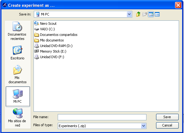
The generation process generates a ZIP file containing all the elements needed to run the experiment. If the experiment generation is completed successfully, the following message will be shown.
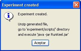
The experiment must be run using the RunKeel jar file located at “experiment/scripts”
In the following picture, we can see an example of the structure of directories that is created. We see that four directories are created:
- exe directory: it contains all the jar files of the algorithms inserted in the experiment.
- scripts directory: it contains the configuration files sorted by algorithm. Also, it contains the RunKeel.jar file which is used in order to run the experiment.
- datasets directory: it contains the datasets used in the experiment. A directory for each dataset is created. Additionally, it will store the results obtained by any of the preprocessed mechanisms selected for the experiment.
- results directory: it contains the output files generated by each algorithm.
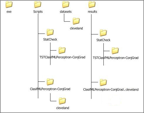
4.7 Menu bar
Each item of the menu bar contains different submenus. These are the different options available:
- File Menu (as shown in Figure 158)
- New Experiment: creates a new experiment.
- Load Experiment: opens an existing experiment. In the open dialog box, select a filename, and click Open. Experiments files usually are saved in XML format.
- Save Experiment: saves the current experiment to a XML file. If it is the first time that the experiment is saved, you will be asked about destination path.
- Save Experiment As: saves current experiment to a XML file. You will be asked about destination path.
- Exit: closes the experiment design tool. If the experiment has not been saved yet, you can do it at this moment.
- View Menu (Figure 159)
- Status Bar: shows/hides the status bar (at the bottom of the windows). Initially, it is active.
- Grid: shows/hides the alignment grid. It helps the user to make easy the alignment of the elements inserted in the draw area. Initially, it is inactive.
- Help Panel: shows/hides the help panel. Initially, it is active.
- DataSets/Algorithm: shows/hides the panel containing the datasets/algorithms. Initially, it is active.
- Edit Menu (Figure 160)
- Undo: with this option the user can undo some actions.
- Redo: with this option user can redo some undone actions.
- Select: allows users to select one or more elements in the draw area.
- Tools Menu (Figure 161)
- Insert Dataflow: allows connecting algorithm outputs (or
dataset) to the inputs of another algorithm, creating a data flow
that will be run later. This option is also available from the left
bar via the button
- Import algorithm KEEL packet: in order to insert a user’s method, select this option and explore the path to choose the method.
- Snapshot: it is possible to save the experiment design into an image format file (JPEG). This way allows you to insert it in any document, article, and so on.
- Run Experiment: when experiment is fully designed, use this option to create a ZIP file containing a directory structure with all the files needed to run the designed experiment in the local computer selected by the user.
- Seed: sets up the value of the seed used by the random number
generator. If there is any algorithm (inserted in the experiment)
that needs to generate random numbers, it will take in a seed
created from the initial seed value. This seed can be established
automatically or you can insert a value manually. The following
picture shows the dialog prompted by this option:
- Execution Options: allows selecting some performance options to
apply to the experiment. In this version, the option defined is the
following:
- Java Heap Size: Indicate the number of MB that will be
allocated in each execution of the algorithm. Default value
is 512MB. Please do not set a higher value than your actual
amount of RAM. The minimum accepted value has been set
to 32MB.
- Java Heap Size: Indicate the number of MB that will be
allocated in each execution of the algorithm. Default value
is 512MB. Please do not set a higher value than your actual
amount of RAM. The minimum accepted value has been set
to 32MB.
- Insert Dataflow: allows connecting algorithm outputs (or
dataset) to the inputs of another algorithm, creating a data flow
that will be run later. This option is also available from the left
bar via the button
- Help Menu (Figure 164)
- Content: show a help dialog that contains information about how to use this program.
- About... : shows a dialog with basic information about the program as name, authors, version, etc...
4.8 Tool bar
To help the user finding the most relevant operations, the KEEL Experiments software tool provides a tool bar with shortcuts to them.
Most of them also appear in the Menu bar (thus, refer to the Menu bar section to get additional information about them). The only option that does not appears already in the Menu bar is:
 Delete: This option allows the user to delete the selected module.
4.9 Status bar
The status bar is a simple way to provide the user useful information during the generation of experiments.
It is located at the bottom of the window. Here it will appear information about the action being carried out, helping the user to understand the meaning of each command or button. Several examples are shown below in Figures 166, 167 and 168:
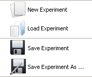
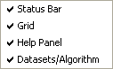
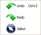
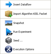
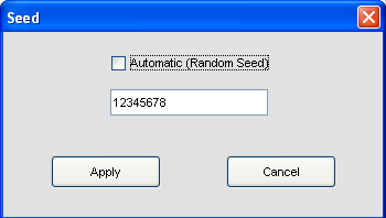
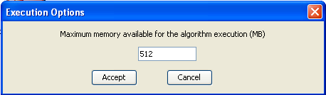


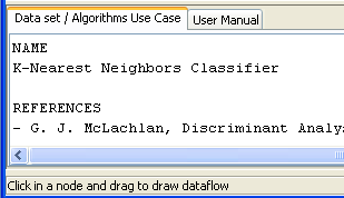
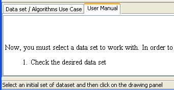
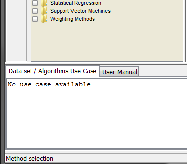
5 Running KEEL Experiments
This section describes the procedure that needs to be followed in order to run and visualize an existing KEEL experiment from the ZIP file generated with the experiment design process.
5.1 Deploying a KEEL experiment
In order to launch a KEEL experiment, an user has to previously design the aforementioned experiment using the KEEL software suite (following the procedure described in Section 4.6). This will create a ZIP file containing all the files needed to run the experiment.
First of all, an user has to unzip the named ZIP file in the machine that will run the experiment (this does not have to be the same machine that was used to create the experiment but needs to be able to run a Java Virtual Machine with at least version 1.7). The user will obtain a directory called “experimentName” (how an user named its experiment). Then, the user has to place himself into that “experimentName” folder, and then into the “scripts” subfolder. To run the experiments, an user just has to type and run the “java -jar RunKeel.jar” command. The experiment is thus executed.
When it finishes, the user will obtain at the command prompt the message “Experiment completed succesfully”.
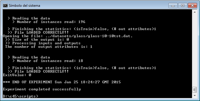
5.2 Viewing the experiment results
Once the run of an experiment has finished, the associated result files can be found at the results\ subdirectory associated to each experiment.
Depending on the type of methods used, the following directories and files will be available:
- Methods: For each combination of method and dataset, there will be
a directory, named <methodName>.<datasetName>.
Inside these directories, the output files generated by the method will have been created (generally, a training and a test output file for each partition, plus every additional output file defined by the method). For further reference, see http://sci2s.ugr.es/keel/outputFiles.php.
- Tests: For each test module employed, a new directory named after the test employed will be available. This directory will contain the output files obtained as a result of the application of the test method.
On the other hand, note that the new datasets obtained as the result of the execution of a preprocessing method will be placed in the datasets\ directory of the experiment, to allow a further employment of them with linked methods in the same experiment.
6 Teaching module
This module has the objective of supporting teachers and students to better understand the working procedure of the Data Mining process for educational purposes. In what follows, we recall the features of the KEEL software and the usage of this particular section.
6.1 Introduction
KEEL is a software tool developed to build and use different Data Mining models. We would like to remark that this is the first software tool of this type containing a free code Java library of Evolutionary Learning Algorithms. The main features of KEEL are:
- It contains pre-processing algorithms: transformation, discretization, instance selections and feature selections.
- It also contains a Knowledge Extraction Algorithms Library, supervised and unsupervised, remarking the incorporation of multiple evolutionary learning algorithms.
- It has a statistical analysis library to analyze algorithms.
- It contains a user-friendly interface, oriented to the analysis of algorithms.
- KEEL’s environment can connect to Internet to download new data files for using them in future analysis.
We can distinguish three parts in the graphic environment:
- The preparation of the dataset part allows users to create different partitions of his own data bases or the data bases available in the KEEL web. Also, it is possible to edit, apply transformations, generate datasets in the correct format from C4.5 files or view detailed plots about a specific dataset.
- The Design of Experiments part has the objective of designing the desired experiments using a graphical interface. After the experiment is designed, the interface generates a .ZIP file containing a directory structure with all the necessary files needed to run those experiments in the local computer
- The Generation of Evolutionary Algorithms with the JCLEC library allows the user to create his own evolutionary algorithms using a graphical interface. In this version of KEEL, this part is NOT implemented.
6.2 Menu Bar
Each item of the menu bar contains different submenus. These are the different options available:
- File Menu
- New Experiment: creates a new experiment. This option is also
available from the tool bar via the button
 .
.
- Load Experiment: opens an existing experiment. In the open
dialog box, select a filename, and click Open. Experiments files
usually have the extension .exp. This option is also available from
the tool bar via the button
 .
.
- Save Experiment: saves the current experiment to a file. If it is
the first time that the experiment is saved, you will be asked
about destination path. This option is also available from the tool
bar via the button
 .
.
- Save Experiment As: saves current experiment in a file. In the save dialog box, introduce the destination path where the file will be saved.
- Exit: closes the experiment design software. If the experiment has not been saved yet, you can do it at this moment.
- New Experiment: creates a new experiment. This option is also
available from the tool bar via the button
- View Menu
- Status Bar: shows/hides the status bar (at the bottom of the windows). It is initially activated.
- Grid: shows/hides the alignment grid. In order to make easy the alignment of the elements inserted in the draw area, it is better to activate it since it will help you to create elegant designs.
- Help Panel: shows/hides the help panel. It is activated initially.
This option is also available from the tool bar via the button
 .
.
- DataSets/Algorithm: shows/hides the panel containing the
datasets/algorithms. It is activated initially. This option is also
available from the tool bar via the button
 .
.
- Edit Menu
- Undo: with this option user can undo some executed actions.
This option is also available from the tool bar via the button
 .
.
- Redo: with this option user can redo some undone actions. This
option is also available from the tool bar via the button
 .
.
- Select: allows users to select one or more elements in the draw
area. This option is also available from the tool bar via the
button
 .
.
- Undo: with this option user can undo some executed actions.
This option is also available from the tool bar via the button
- Tools Menu
- Insert Dataflow: allows connecting algorithm outputs (or
dataset) to the inputs of another algorithm, creating a data flow
that will be run later. This option is also available from the tool
bar via the button
- Import algorithm KEEL packet: in order to insert a user’s method, select this option and explore the path to choose the method.
- Snapshot: it is possible to save the experiment design in an
image format file (JPEG). This way allows you to insert it in any
document, article, etc... This option is also available from the tool
bar via the button

- Run Experiment: when experiment is finished, use this option to
create a ZIP file containing a directory structure with all the files
needed to run the designed experiment in the local computer
selected by the user. This option is also available from the tool
bar via the button
 .
.
- Seed: sets up the value of the seed used by the random number
generator. If there is any algorithm (inserted in the experiment)
that needs to generate random numbers, it will take in a seed
created from the initial seed value. This seed can be established
automatically or you can insert a value manually. This is shown
at the following picture (Figure 170):
- Insert Dataflow: allows connecting algorithm outputs (or
dataset) to the inputs of another algorithm, creating a data flow
that will be run later. This option is also available from the tool
bar via the button
- Help Menu
- Content: show a help dialog that contains information about how to use this program.
- About... : shows a dialog with basic information about the program as name, authors, version, and so on.
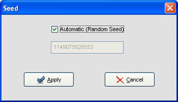
6.3 Tools Bar
There are two tool bars in this program. One of them appears under the menu bar. Pressing on its buttons it is possible to access to the most frequently used options that appear in the menus. It looks like Figure 171:
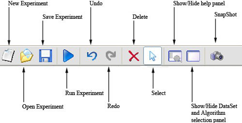
The other one is located on the left of the main window, and it contains buttons to perform specific options of design. It looks like the one shown in Figure 172:
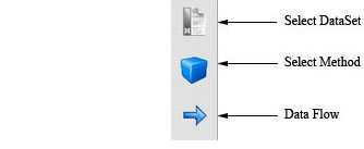
If you put the mouse over a button, it will appear a short description about it.
6.4 Status Bar
The status bar is located at the bottom of the window (Figure 173). Here it will appear information about the action being carried out, helping the user to understand the meaning of each command or button.

6.5 Experiment Graph
6.5.1 Datasets
- Insert dataset: in order to insert a dataset, we must perform the
following steps:
- Choose the desired datasets from the “Select Datasets” panel on
the left of the window (Figure 174).
At this point, you can import an existing KEEL dataset into your current KEEL datasets selection. Just click in the
 button. The next
windows will appear (Figure 175):
button. The next
windows will appear (Figure 175):
Once you have selected your new datasets, they will appear under the default KEEL dataset selection (please refer to User Datasets section 3.1.2), and your previous dataset selection will be kept, as shown in Figure 176.
- Click on the draw area.
Once again, you can import new datasets in this step, by clicking in
button
- Choose the desired datasets from the “Select Datasets” panel on
the left of the window (Figure 174).
- Configure dataset: once the dataset is inserted, we can indicate which
partitions (training and test) we want to use. To do so, click on the
 button near the dataset’s name and the following dialog appears (Figure
177).
button near the dataset’s name and the following dialog appears (Figure
177).
Initially, this dialog has the entire file. So, if you want to remove some of them, select it and then click the
 button. Another way is
to remove all the files by clicking the
button. Another way is
to remove all the files by clicking the  button, and then add
the files you want. To do that, you must look for the training and
test file by clicking the
button, and then add
the files you want. To do that, you must look for the training and
test file by clicking the  button and, after that, click the
  button.
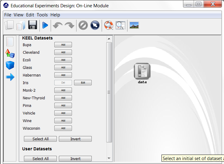
6.5.2 Algorithms
- Types
There exist several types of algorithms according to their functionality. Let us see as they are:
- Pre-process: they are discretization algorithms, instances
selection and features selection. As their name suggests, they
are used to add a pre-processing step over the initial dataset,
before applying a knowledge extraction algorithm. The list of
algorithms is shown in Figure 178.
For each category there exist the following algorithms:
- Discretizers
- Fayyad
- Uniform FrequencyUniform Width
- Training set selection (standard and evolutionary)
- ENN
- CHC
- GGA
- SGA
- Feature Selection
- LVF
- Relief
- Discretizers
- Methods: user may find several knowledge extraction algorithms
such as decision trees and rule extraction, neural networks, support
vector machines, and so on. The complete list is shown in Figure
179.
For each category there exist the following algorithms:
- Statistical Methods
- LDA
- LinearLMS (Classification and Regression)
- NaiveBayes
- Fuzzy Rule Learning (standard and evolutionary)
- Chi-RW
- Wang and Mendel
- GFS-GP
- MOGUL
- Thrift
- Decision Trees
- C45
- CART
- M5
- Neural Networks
- Perceptron with Conjugate gradient (classification and regression)
- Radial Base Function Network (classification and regression)
- iRProp+
- Crisp Rule Learning:
- PGIRLA
- XCS
- Lazy Learning
- KNN
- Support Vector Machines
- C_SVM
- EPSILON_SVR
- Statistical Methods
- Pre-process: they are discretization algorithms, instances
selection and features selection. As their name suggests, they
are used to add a pre-processing step over the initial dataset,
before applying a knowledge extraction algorithm. The list of
algorithms is shown in Figure 178.
- Insert Algorithm
In order to add an algorithm to our experiment, we must perform the following actions (Figure 180):
- Select the desired option from the tool bar on the left, according to the type of algorithm we want to insert: pre-process, method.
- Choose the desired algorithm from the tree structure.
- Click on the draw area.
- Algorithm Parameters Configuration
Once the algorithm has been inserted, we can configure the value of its parameters. To do so, you must double click on the algorithm symbol and a dialog is shown (Figure 181).
At the top of this dialog we can indicate the number of times we want to run the algorithm (only available for random methods). Each execution will be made using a seed generated from the initial seed.
In the table located in the center of the window, it appears all algorithm parameters established to its initial values. You can modify them as you wish. If you want to return to initial values, press the
 button.
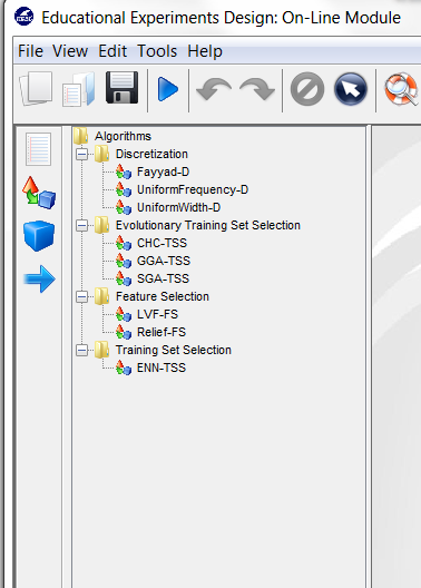
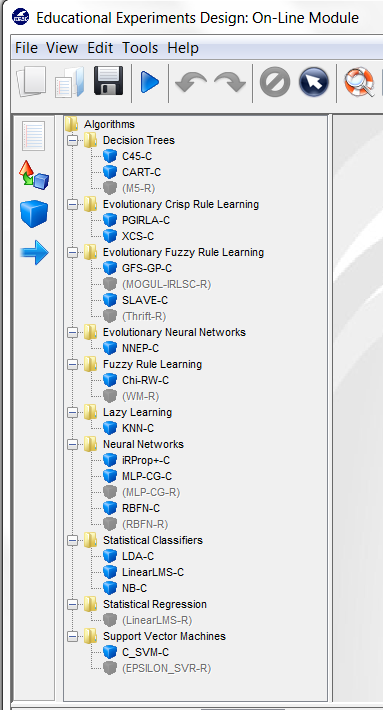
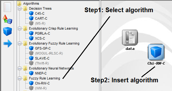
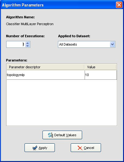
6.5.3 Connections
They allow you to connect algorithm outputs (or dataset) to the inputs of another algorithm, creating a data flow that will be run later.
- Insert connection: to make a connection, select the button from
the left tool bar. Then, click on the source node and finally click on the
target node.
- Restrictions: there are some restrictions that must be considered when
making connections between the different elements:
- A dataset cannot have inputs.
- Knowledge extraction methods can receive data from a dataset or from a previous method.
- The graph cannot have any cycle.
All these restrictions are verified in execution time when a connection is been created. If one of these connections is not permitted, the application will show an error message. In next figures you can see some examples of incorrect graphs.
6.5.4 Inteface Management
In this section we will see some additional considerations about other possibilities that provide this application.
- Parameters configuration menu: it is possible to access to the parameters configuration context menu of an algorithm by double-clicking with the mouse on a certain method node in the draw area.
- Objects selection: in order to select a single element, just click with the left button of the mouse over it. But if we want to select several elements, we click in an empty zone of the draw area and drag the mouse until covering all the objects we wish to select. Finally we release the button and we get elements selected.
- Move objects: we can move one or several elements selected with the aid of the left button of the mouse. You just have to click over the selected objects and, without release the button, drag them to the desired position. Another way is to use the keyboard cursors.
- Remove objects: in order to delete one or more objects from the graph
we must select them and press the button of the upper tool bar.
- Undo - Redo: we can undo or redo the performed actions through the
and buttons of the upper tool bar.
- Snapshots: it is possible to save the experiment design in an image
format file (JPEG). Using this option you will be able to insert it in
any document, article, etc... This option is available through the
button of the upper tool bar.
7 KEEL Modules
In this section, we introduce several modules that are included in KEEL for particular purposes. Specifically, three different modules have been developed:
- A complete section devoted to classification with imbalanced datasets, taking into account the special features of this scenario.
- A statistical software for the proper validation of the results obtained in the experimental studies.
- A full semi-supervised learning module that provides some representative datasets and the state-of-the-art of self-labeling algorithms.
- A module for multiple instance learning, including datasets and algorithms for this type of classification task.
All these modules are described throughout the following sections.
7.1 Imbalanced Learning Module
In many supervised learning applications, there is a significant difference between the prior probabilities of different classes. This situation is known as the class imbalance problem and it is common in many real problems from telecommunications, web, finance-world, ecology, biology, medicine and so on. In this way, it has been considered as one of the top problems in data mining today. Furthermore, it is worth to point out that the minority class is usually the one that has the highest interest from a learning point of view and it also implies a great cost when it is not well classified.
The KEEL Software Suite have taken into account this significant scenario of classification and it includes a complete framework for the experimentation of this type of problems. In this section, we will briefly introduce the features of classification with imbalanced datasets and we will describe how this is addressed with KEEL.
7.1.1 Introduction to classification with imbalanced datasets
The hitch with imbalanced datasets is that standard classification learning algorithms are often biased towards the majority class (known as the “negative” class) and therefore there is a higher misclassification rate for the minority class instances (called the “positive” examples). Since most of the standard learning algorithms consider a balanced training set, this may generate suboptimal classification models, i.e. a good coverage of the majority examples, whereas the minority ones are misclassified frequently. Therefore, those algorithms, which obtain a good behavior in the framework of standard classification, do not necessarily achieve the best performance for imbalanced datasets. There are several reasons behind this behavior:
- The use of global performance measures for guiding the learning process, such as the standard accuracy rate, may provide an advantage to the majority class.
- Classification rules that predict the positive class are often highly specialized and thus their coverage is very low, hence they are discarded in favor of more general rules, i.e. those that predict the negative class.
- Very small clusters of minority class examples can be identified as noise, and therefore they could be wrongly discarded by the classifier. On the contrary, few real noisy examples can degrade the identification of the minority class, since it has fewer examples to train with.
Therefore, throughout the last years, many solutions have been proposed to deal with this problem, both for standard learning algorithms and for ensemble techniques. They can be categorized into three major groups:
- Data sampling: In which the training instances are modified in such a way to produce a more or less balanced class distribution that allow classifiers to perform in a similar manner to standard classification.
- Algorithmic modification: This procedure is oriented towards the adaptation of base learning methods to be more attuned to class imbalance issues.
- Cost-sensitive learning: This type of solutions incorporate approaches at the data level, at the algorithmic level, or at both levels combined, considering higher costs for the misclassification of examples of the positive class with respect to the negative class, and therefore, trying to minimize higher cost errors.
Most of the studies on the behavior of several standard classifiers in imbalance domains have shown that significant loss of performance is mainly due to the skewed class distribution, given by the imbalance ratio (IR), defined as the ratio of the number of instances in the majority class to the number of examples in the minority class.
In imbalanced domains, the evaluation of the classifiers’ performance must be carried out using specific metrics in order to take into account the class distribution. Particularly, four metrics can be employed for computing the classification performance of both, positive and negative, classes independently:
- True positive rate: TPrate =
 is the percentage of positive
instances correctly classified.
is the percentage of positive
instances correctly classified.
- True negative rate: TNrate =
 is the percentage of negative
instances correctly classified.
is the percentage of negative
instances correctly classified.
- False positive rate: FPrate =
 is the percentage of negative
instances misclassified.
is the percentage of negative
instances misclassified.
- False negative rate: FNrate =
 is the percentage of positive
instances misclassified.
is the percentage of positive
instances misclassified.
Since in this classification scenario we intend to achieve good quality results for both classes, there is a necessity of combining the individual measures of both the positive and negative classes, as none of these measures alone is adequate by itself.
A well-known approach to unify these measures and to produce an evaluation
criteria is to use the Receiver Operating Characteristic (ROC) graphic. This
graphic allows the visualization of the trade-off between the benefits (TPrate) and
costs (FPrate), as it evidences that any classifier cannot increase the number of true
positives without also increasing the false positives. The Area Under the ROC
Curve (AUC) corresponds to the probability of correctly identifying
which one of the two stimuli is noise and which one is signal plus noise.
The AUC provides a single measure of a classifier’s performance for
evaluating which model is better on average. Figure 184 shows how
to build the ROC space plotting on a two-dimensional chart the TPrate
(Y-axis) against the FPrate (X-axis). Points in (0,0) and (1,1) are trivial
classifiers where the predicted class is always the negative and positive one,
respectively. On the contrary, (0,1) point represents the perfect classifier. The
AUC measure is computed just by obtaining the area of the graphic as
AUC = 
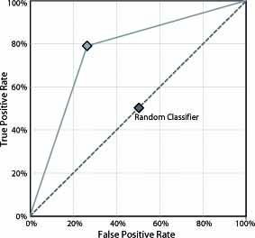
Apart from the AUC measure, it is also commmon to use the geometric mean (GM) of the true positive and true negative rates (TPrate and TNrate) obtained by the classifier and is given by
 | (1) |
7.1.2 Imbalanced Experiments Design: Offline module
In order to have access to this part of the software, in the first frame of the program we must click on Modules, and then select Imbalanced Learning as shown in Figure 185.
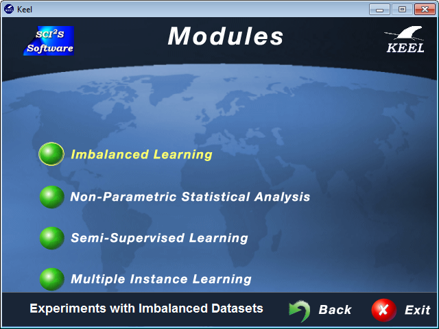
Once we have clicked, a new window will appear, with the same appearance that the standard “Design of Experiments” framework (please refer to Section 4.3). Regarding to this fact, all menu bars include exactly the same patterns, i.e. the menu, tool, and status bars.
In fact, all the process for preparing an experiment follows the same scheme than in the standard “Offline experiments” module, which has been described throughout sections 4.3, 4.4 and 4.6. However, we must point out several significant differences between both scenarios, regarding the Experimental Graph: (1) Datasets, (2) Preprocessing methods, (3) Algorithms, and (4) Statistical tests and Visualization:
- Datasets
There is no consensus in the research community on what threshold must be set up for a given dataset to suffer from the imbalance problem. For KEEL Software Suite, a dataset is considered to be imbalanced when the positive class has a distribution of examples below 40% of the number of instances that belong to the majority class. In other words, the ratio between the examples of the majority and minority class should be higher than 1.5.
In particular, 44 binary datasets have been included by default within the software. These datasets have been generated by modifying multi-class problems to obtain binary imbalanced problems. In particular, this collection of benchmark problems have been widely used in the specialized literature for classification with imbalanced data. Together with the name of the problem, the specific IR of each one of them is noted between brackets. Therefore, problems are ordered according to this value, as shown in Figure 186.
Two different partitioning schemes are allowed: 5-fold stratified cross validation and Distribution optimally balanced stratified cross-validation (DOB-SCV). The user can choose the validation scheme in the drop menu that is above the list of available datasets (See Figure 186). By default, the 5-fold stratified cross validation is selected. See Section 7.1.2 for more details.
As in the case of the basic KEEL Experiment section, we must select those problems we want to work with, and then click over the experimental panel (Figure 187). Now we are able to choose from the set of preprocessing methods and classification algorithms.
- Preprocessing
Apart from the preprocessing techniques included in the KEEL Experiment section, this module includes two new categories: Over-Sampling Methods and Under-Sampling techniques. Both methodologies appear highlighted in boldface in the list of preprocessing models available.
As previously stated in section 7.1.1, data sampling via preprocessing techniques is one of the most common approaches for dealing with skewed data distribution. In this way, the original training set can be modified by oversampling the minority class examples (by replication or generation of synthetic data), or undersampling the majority class examples.
KEEL Software Suite includes the state-of-the-art for both types of techniques. This list of techniques is summarized in Figure 188:
- Oversampling techniques
- ADASYN
- Adjusting the Direction Of the synthetic Minority clasS examples (ADOMS)
- Aglomerative Hierarchical Clustering (AHC)
- Borderline SMOTE
- Random over-sampling
- Safe Level SMOTE
- Synthetic Minority Over-sampling Technique (SMOTE)
- SMOTE (Synthetic Minority Over-sampling Technique) + ENN (Edited Nearest Neighbor)
- SMOTE-RSB*: Preprocessing using SMOTE and Rough Sets Theory
- SMOTE (Synthetic Minority Over-sampling Technique) + Tomek Links
- SPIDER
- SPIDER2
- Undersampling techniques
- Condensed Nearest Neighbor (CNN)
- Condensed Nearest Neighbor + Tomek’s modification of Condensed Nearest Neighbor
- Class Purity Maximization (CPM)
- Neighborhood Cleaning Rule
- One Sided Selection
- Random under-sampling
- Undersampling Based on Clustering
- Tomek’s modification of Condensed Nearest Neighbor
- Oversampling techniques
- Methods
A large number of approaches have been proposed to deal with the class imbalance problem. These approaches can be categorized into two groups: the internal approaches that create new algorithms or modify existing ones to take the class-imbalance problem into consideration and external approaches that preprocess the data in order to diminish the effect of their class imbalance.
Furthermore, cost-sensitive learning solutions incorporating both the data (external) and algorithmic level (internal) approaches assume higher misclassification costs for samples in the minority class and seek to minimize the high cost errors. Ensemble methods are also frequently adapted to imbalanced domains, either by modifying the ensemble learning algorithm at the data-level approach to preprocess the data before the learning stage of each classifier or by considering to embed a cost-sensitive framework in the ensemble learning process.
In addition to the preprocessing mechanisms for addressing the skewed data distribution (external approaches), within the KEEL Imbalanced Learning Module we may find three main categories: Algorithmic Modifications for Class Imbalance Cost-sensitive classification and Ensemble for class imbalance. For the sake of clarity, these three categories have been stressed in boldface, as shown in Figure 189.
The list of implemented algorithms is given below:
- Cost-Sensitive Classification
- C-SVM for Classification Cost-Sensitive
- C4.5 Cost Sensitive Decision Tree
- Multilayer perceptron for Cost-Sensitive classification problems
- Ensembles for Class-Imbalance
- AdaBoost algorithm with C4.5 Decision Tree as Base Classifier
- AdaBoost.M1 algorithm with C4.5 Decision Tree as Base Classifier
- AdaBoost.M2 algorithm with C4.5 Decision Tree as Base Classifier
- Cost Sensitive Boosting with C4.5 Decision Tree as Base Classifier
- Bagging algorithm with C4.5 Decision Tree as Base Classifier
- BalanceCascade ensemble with C4.5 Decision Tree as Base Classifier
- DataBoost-IM algorithm with C4.5 Decision Tree as Base Classifier
- EasyEnsemble with C4.5 Decision Tree as Base Classifier
- IIVotes: SPIDER + IVotes with C4.5 Decision Tree as Base Classifier
- MSMOTEBagging with C4.5 Decision Tree as Base Classifier
- MSMOTEBoost with C4.5 Decision Tree as Base Classifier
- OverBagging algorithm with C4.5 Decision Tree as Base Classifier
- OverBagging2 algorithm with C4.5 Decision Tree as Base Classifier
- RUSBoost algorithm with C4.5 Decision Tree as Base Classifier
- SMOTEBagging algorithm with C4.5 Decision Tree as Base Classifier
- SMOTEBoost algorithm with C4.5 Decision Tree as Base Classifier
- UnderBagging algorithm with C4.5 Decision Tree as Base Classifier
- UnderBagging2 algorithm with C4.5 Decision Tree as Base Classifier
- UnderOverBagging algorithm with C4.5 Decision Tree as Base Classifier
- Cost-Sensitive Classification
- Visualization and Statistical Tests
This part of the software follows the same scheme that for standard classification, as described in Sections 4.3.5 and 4.3.6. The main difference between both scenarios, is that in this case the performance is computed by means of the AUC or the GM metrics, which were previously introduced in Section 7.1.1.
Additionally, only non-parametrical statistical tests are available in this current case, namely the Wilcoxon pairwise test and the Friedman Test and Post-Hoc Procedures (Figure 190). In the latter case, we may choose among Iman and Davenport test, Bonferroni-Dunn test, Holm test, Hochbergh test, Hommel test, Holland test, Rom test, Finner test or Li test.
Regarding the visualization part, the procedures are the same, just differing, as stated above, in the metric of performance that is taken into account, i.e. the AUC metric (Figure 191).
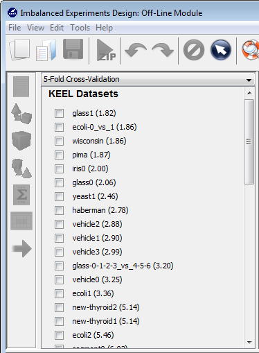
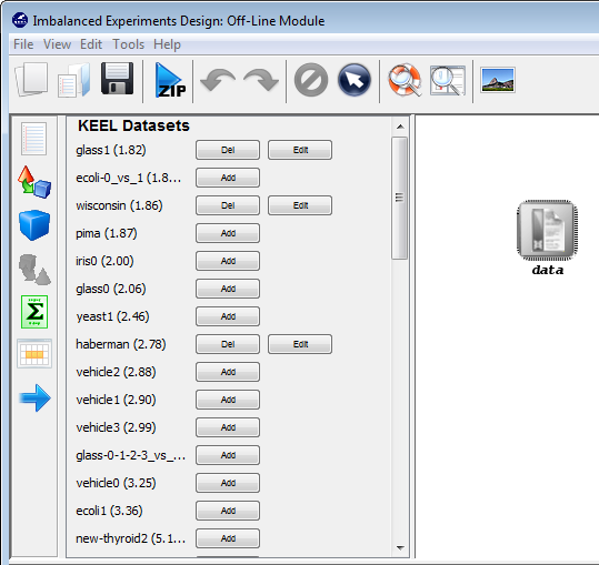
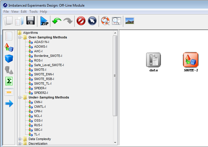
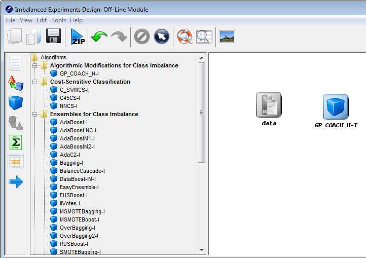
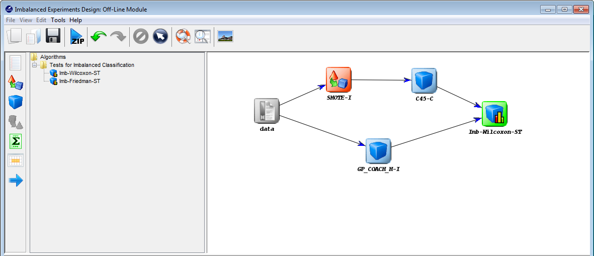
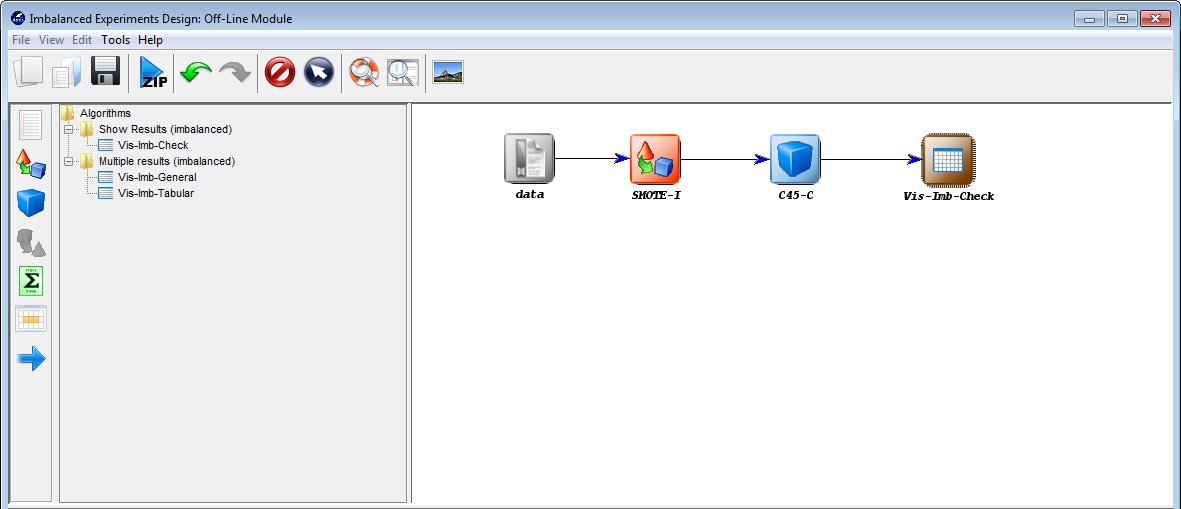
7.2 Statistical tests Module
The goodness of a given approach cannot be only measured in terms of the improvement for the mean performance. Significant differences must be found among the different algorithms for concluding the superior behavior of the one that achieves the highest average result.
For this reason, in KEEL Software Suite several hypothesis testing techniques are included in order to provide statistical support for the analysis of the results.
Specifically, we will use non-parametric tests, due to the fact that the initial conditions that guarantee the reliability of the parametric tests may not be satisfied, causing the statistical analysis to lose credibility with these type of tests. Any interested reader can find additional information on the Website http://sci2s.ugr.es/sicidm/.
7.2.1 Introduction to statistical test
The experimental analysis on the performance of a new method is a crucial and necessary task to carry out in a research on Data Mining, Computational Intelligence techniques. Deciding when an algorithm is better than other one may not be a trivial task.
Hyphotesis testing and p-values: In inferential statistics, sample data are primarily employed in two ways to draw inferences about one or more populations. One of them is the hypothesis testing.
The most basic concept in hypothesis testing is a hypothesis. It can be defined as a prediction about a single population or about the relationship between two or more populations. Hypothesis testing is a procedure in which sample data are employed to evaluate a hypothesis. There is a distinction between research hypothesis and statistical hypothesis. The first is a general statement of what a researcher predicts. In order to evaluate a research hypothesis, it is restated within the framework of two statistical hypotheses. They are the null hypothesis, represented by the notation H0, and the alternative hypothesis, represented by the notation H1.
The null hypothesis is a statement of no effect or no difference. Since the statement of the research hypothesis generally predicts the presence of a difference with respect to whatever is being studied, the null hypothesis will generally be a hypothesis that the researcher expects to be rejected. The alternative hypothesis represents a statistical statement indicating the presence of an effect or a difference. In this case, the researcher generally expects the alternative hypothesis to be supported.
An alternative hypothesis can be nondirectional (two-tailed hypothesis) and directional (one-tailed hypothesis). The first type does not make a prediction in a specific direction; i.e. H1 : μ ≠ 100. The latter implies a choice of one of the following directional alternative hypothesis; i.e. H1:μ 100 or H1:μ 100.
Upon collecting the data for a study, the next step in the hypothesis testing procedure is to evaluate the data through use of the appropriate inferential statistical test. An inferential statistical test yields a test statistic. The latter value is interpreted by employing special tables that contain information with regard to the expected distribution of the test statistic. Such tables contain extreme values of the test statistic (referred to as critical values) that are highly unlikely to occur if the null hypothesis is true. Such tables allow a researcher to determine whether or not the results of a study is statistically significant.
The conventional hypothesis testing model employed in inferential statistics assumes that prior to conducting a study, a researcher stipulates whether a directional or nondirectional alternative hypothesis is employed, as well as at what level of significance is represented the null hypothesis to be evaluated. The probability value which identifies the level of significance is represented by ?.
When one employs the term significance in the context of scientific research, it is instructive to make a distinction between statistical significance and practical significance. Statistical significance only implies that the outcome of a study is highly unlikely to have occurred as a result of chance, but it does no necessarily suggest that any difference or effect detected in a set of data is of any practical value. For example, no-one would normally care if algorithm A in continuos optimization solves the sphere function to within 10-10 of error of the global optimum and algorithm B solves it within 10-15. Between them, statistical significance could be found, but in practical sense, this difference is not significant.
Instead of stipulating a priori a level of significance ?, one could calculate the smallest level of significance that results in the rejection of the null hypothesis. This is the definition of p-value, which is an useful and interesting datum for many consumers of statistical analysis. A p-value provides information about whether a statistical hypothesis test is significant or not, and it also indicates something about how significant the result is: The smaller the p-value, the stronger the evidence against the null hypothesis. Most important, it does this without committing to a particular level of significance.
The most common way for obtaining the p-value associated to a hypothesis is by means of normal approximations, that is, once computed the statistic associated to a statistical test or procedure, we can use a specific expression or algorithm for obtaining a z value, which corresponds to a normal distribution statistics. Then, by using normal distribution tables, we could obtain the p-value associated with z.
7.2.2 KEEL Suite for Statistical Analysis
In order to have access to this part of the software, in the first frame of the program we must click on Modules, and then select Non-Parametric Statistical Analysis as shown in Figure 192.

Once we have clicked, a new window will appear. This module allows to perform several non-parametric statistical test over a given set of results. Further information about them can be found in the SCI2S thematic Web Site of Statistical Inference in Computational Intelligence and Data Mining http://sci2s.ugr.es/sicidm/
In this version, the available procedures are the following:
- Friedman test.
- Quade test.
- Friedman Alligned test.
- Friedman test NxN (Multiple test).
- Contrast estimation (contrast estimation based on medians).
- Wilcoxon signed-ranks test.
They can be selected through the Statistical procedures box:
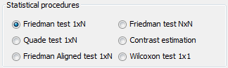
Post hoc methods
In order to characterize the differences detected by the statistical tests, this module also provides a set of well-known post hoc methods.
For Friedman, Quade and Friedman alligned tests, it is possible to employ the following post hoc tests:
- Iman-Davenport.
- Bonferroni-Dunn.
- Holm.
- Hochberg.
- Hommel.
- Holland.
- Rom.
- Finner.
- Li.
For multiple tests, it is possible to employ the following post hoc tests:
- Iman-Davenport.
- Holm.
- Nemenyi.
- Shaffer.
- Bergman.
Performance measure
Depending on the characteristics of the problem considered, it is possible to perform the statistical test for maximization and minimization problems.
This feature allows to determine if the results have been obtained from a maximization problem (e.g. using accuracy in supervised classification problems) or from a minimization problem (e.g. using MS Error in regression problems).
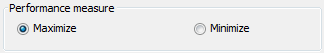
Working with data
The data table stores the average results achieved by each algorithm in each data set (problem). See Figure 195.
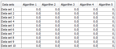
It is possible to input the values directly on the cells of the table, updating both results and the names of the data sets (however, algorithms’ names can only be updated through reading a CSV results file, see the next section). See Figure 196.
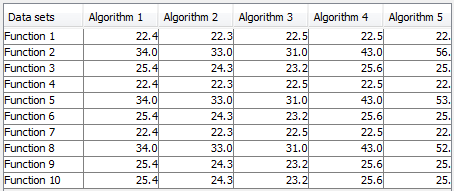
Table controls
The following operations are defined to manage the data table (Figure 197).
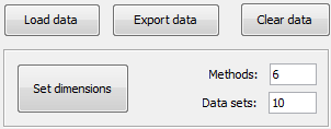
- Load data: Load data in the table from a CSV file. The format defined
is the following (Figure 198).
That is, algorithms are expressed in columns, whereas problems are defined in rows. Only , and ; are allowed as separators. Note that, if desired, this is the way to change algorithms’ names in the table.
- Export data: Exports the data stored in the table in a CSV file (in the same format that has been explained in the Load data section).
- Clear data: Cleans the data table, setting all values to default.
- Set dimensions: Defines the number of rows (data sets) and columns (algorithms) of the table. When this option is used, the data table is also cleaned completely.
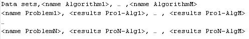
Generation of analysis
Finally, when the data table has been filled with the results to analyze, and all the relevant options have been selected, the analysis can be performed through the Perform Analysis button (Figure 199).

The name for a .tex (a LaTeX file) will be needed to store the results of the analysis. Then, if the data introduced is correct, the analysis will be performed (Figure 200).
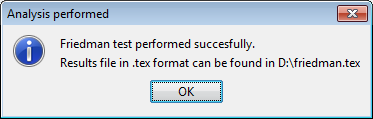
This .tex file contains all the information offered by the tests. To revise it, just compile the file with your favourite LaTeX processor, in order to obtain a PDF/PS/DVI file containing the results.
7.3 Semi-supervised Learning Module
The Semi-Supervised Learning (SSL) paradigm has attracted much attention in many different fields ranging from bioinformatics to web mining, where it is easier to obtain unlabeled than labeled data because it requires less effort, expertise and time-consumption. In this context, traditional supervised learning is limited to using labeled data to build a model. Nevertheless, SSL is a learning paradigm concerned with the design of models in the presence of both labeled and unlabeled data. Essentially, SSL methods use unlabeled samples to either modify or reprioritize the hypothesis obtained from labeled samples alone.
The KEEL Software Suite have taken into account this significant scenario of classification and it includes a complete framework for the experimentation of this type of problems. In this section, we will briefly introduce the features of semi-supervised classification and we will describe how this is addressed with KEEL.
7.3.1 Semi-supervised Learning Experiments Design: Offline module
In order to have access to this part of the software, in the first frame of the program we must click on Modules, and then select Semi-supervised Learning as shown in Figure 201.
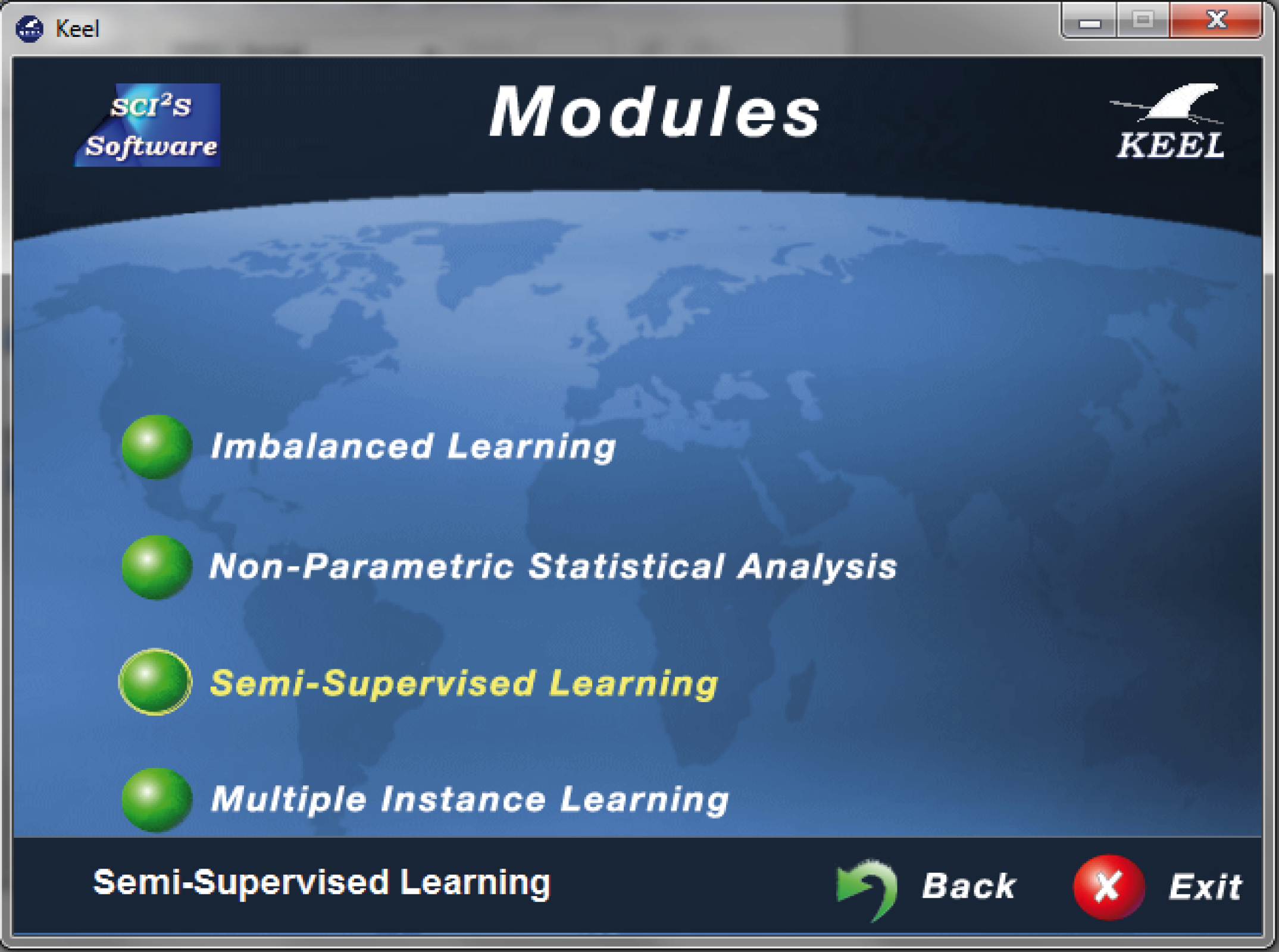
Once we have clicked, a new window will appear, with the same appearance that the standard “Design of Experiments” framework (please refer to Section 4.3). Regarding to this fact, all menu bars include exactly the same patterns, i.e. the menu, tool, and status bars.
In fact, all the process for preparing an experiment follows a very similar scheme than in the standard “Offline experiments” module, which has been described throughout sections 4.3, 4.4 and 4.6. However, we must point out several significant differences between both scenarios, regarding the Experimental Graph: (1) Datasets, and (2) Preprocessing and (3) Algorithms:
- Datasets
In semi-supervised classification we work with both unlabeled and labeled examples. Firstly, we perform a 10-fold cross-validation procedure diving into training and test sets. It is noteworthy that test partitions are kept aside to evaluate for inductive purposes.
The training partitions have been divided into labeled and unlabeled examples. In the division process we do not maintain the class proportion in the labeled and unlabeled sets since the main aim of semi-supervised classification is to exploit unlabeled data for better classification results. Hence, we use a random selection of examples that will be marked as labeled instances, and the class label of the rest of the instances will be removed.
Different labeled ratios can be considered. Within the KEEL-dataset repository, we can find: 10, 20, 30 and 40 %. Thus, for instance, assuming a data set that contains 1,000 examples, when the labeled rate is 10 %, 100 examples are put into the labeled set with their labels, while the remaining 900 examples are put into the unlabeled set without their labels.
Several SSL problems with 10% of labeled ratio have been included within KEEL, as shown in Figure 202.
As in the case of the basic KEEL Experiment section, we must select those problems we want to work with, and then click over the experimental panel (Figure 203). Now we are able to choose from the set of preprocessing methods and classification algorithms.
- Preprocessing
In this case, no preprocessing techniques have been added into the software. Nevertheless, the software is ready to add this kind of techniques, such as Feature selection, dimensionality reduction, etc.
- Methods
For the SSL KEEL module, the state-of-the-art in self-labeling techniques have been included. Moreover, for comparison purposes, some standard classification techniques: C4.5, Naive Bayes, Neural Networks and SVM have been also added to be run on SSL methods. In this way, these methods do not use unlabeled examples to use them as baseline comparison models.
The list of SSL models is shown in Figure 204:
- Multiple-classifiers:
- ADE_CoForest
- CLCC
- Co-Bagging(CoBC)
- CoForest
- Co-Training
- DE-TriTraining
- Democratic-Co
- Random subspace method for co-training
- (RASCO)
- Rel-RASCO
- Tri-Training.
- Single-classifiers:
- APSSC
- Self-Training
- SETRED
- Self-training nearest neighbor rule using cut edges (SNNRCE)
- Multiple-classifiers:
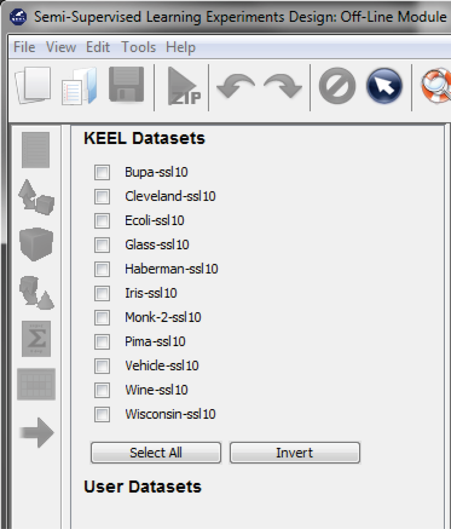
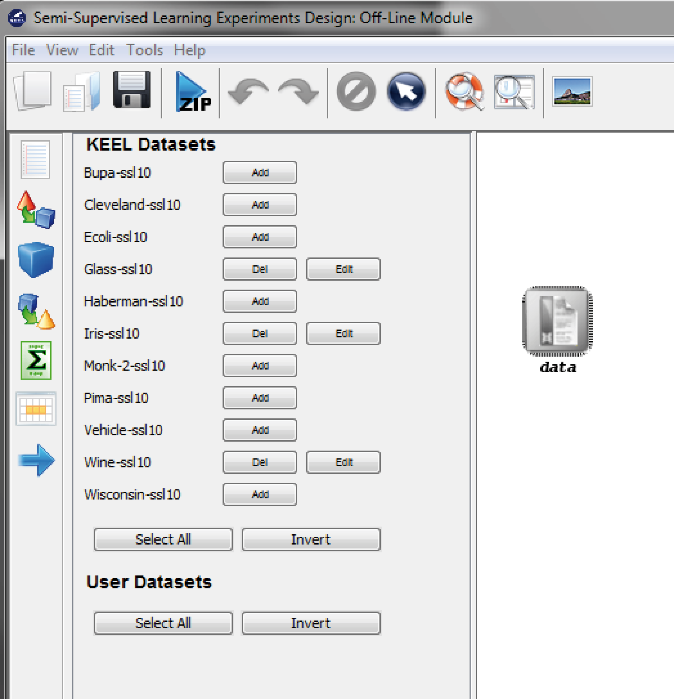
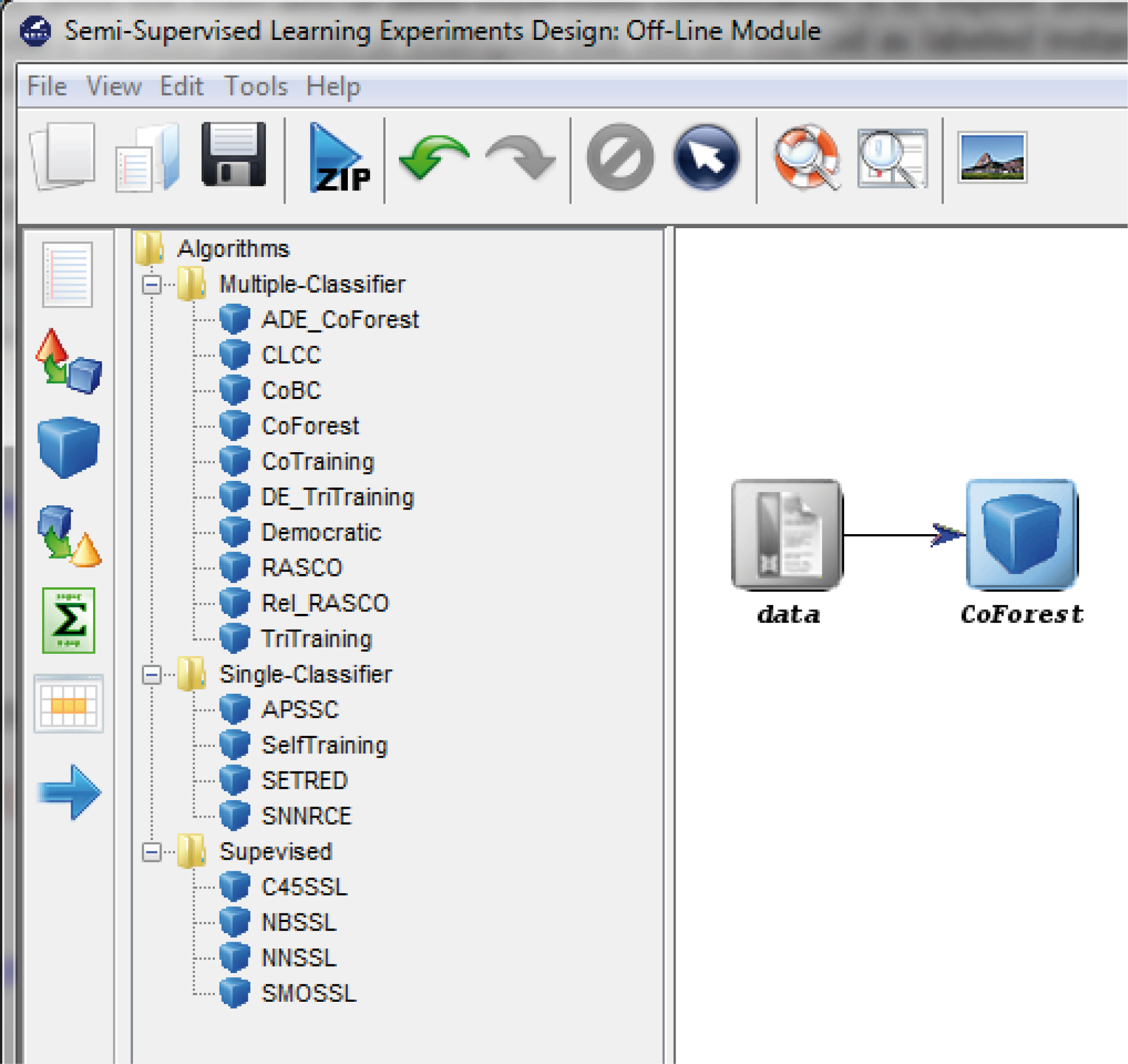
7.4 Multiple Instance Learning Module
Multiple instance learning (MIL) is a generalization of traditional supervised learning. In MIL, training patterns called bags are represented as a set of feature vectors called instances. Each bag contains a number of non-repeated instances and each instance usually represents a different view of the training pattern attached to it. There is information about the bags and each one receives a special label, although the labels of instances are unknown. The problem consists of generating a classifier that will correctly classify unseen bags of instances. The key challenge in MIL is to cope with the ambiguity of not knowing which instances in a positive bag are actually positive examples, and which ones are not. In this sense, a multiple instance learning problem can be regarded as a special kind of supervised learning problem with incomplete labeling information
The KEEL Software Suite have taken into account this significant scenario of classification and it includes a complete framework for the experimentation of this type of problems. In this section, we will briefly introduce the features of classification with multiple instance data and we will describe how this is addressed with KEEL.
7.4.1 Introduction to multiple instance learning
MIL is designed to solve the same problems as single-instance learning: learning a concept that correctly classifies training data as well generalizing unseen data. Although the actual learning process is quite similar, the two approaches differ in the class labels provided which are what they learn from. In a traditional machine learning setting, an object mi is represented by a feature vector vi, which is associated with a label f(mi). However, in the multiple instance setting, each object mi may have Vi various instances denoted mi1, mi2, …, mivi . Each of these variants will be represented by a (usually) distinct feature vector V(mi,j). A complete training example is therefore written as ({V(mi,1), V(mi,2), …, V(mi,vi)}, f(mi)).
The goal of learning is to find a good approximation to the function f(mi),
 (mi), analyzing a set of training examples and labeled as f(mi). To obtain this
function Dietterich defines a hypothesis that assumes that if the result observed
is positive, then at least one of the variant instances must have produced that
positive result. Furthermore, if the result observed is negative, then none of the
variant instances could have produced a positive result. This can be modeled by
introducing a second function g(V(mi,j)) that takes a single variant instance and
produces a result. The externally observed result, f(mi), can then be defined as
follows:
(mi), analyzing a set of training examples and labeled as f(mi). To obtain this
function Dietterich defines a hypothesis that assumes that if the result observed
is positive, then at least one of the variant instances must have produced that
positive result. Furthermore, if the result observed is negative, then none of the
variant instances could have produced a positive result. This can be modeled by
introducing a second function g(V(mi,j)) that takes a single variant instance and
produces a result. The externally observed result, f(mi), can then be defined as
follows:

7.4.2 Multiple Instance Learning Experiments Design: Offline module
In order to have access to this part of the software, in the first frame of the program we must click on Modules, and then select Multiple Instance Learning as shown in Figure 185.
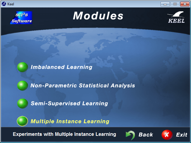
Once we have clicked, a new window will appear, with the same appearance that the standard “Design of Experiments” framework (please refer to Section 4.3). Regarding to this fact, all menu bars include exactly the same patterns, i.e. the menu, tool, and status bars.
In fact, all the process for preparing an experiment follows the same scheme than in the standard “Offline experiments” module, which has been described throughout sections 4.3, 4.4 and 4.6. However, we must point out several significant differences between both scenarios, regarding the Experimental Graph: (1) Datasets, (2) Preprocessing methods, and (3) Algorithms:
- Datasets
Although MIL is a relatively recent learning framework, the MIL setting has produced numerous and interesting applications in different domains which have improved considerably the previous results achieved with other learning frameworks due to greater flexibility in their representation. In KEEL software, a drug activity prediction problem (musk dataset) has been considered by default, as shown in Figure 206. This dataset has been previously partitioned following a 10 fold cross validation scheme.
As in the case of the basic KEEL Experiment section, we must select those problems we want to work with, and then click over the experimental panel (Figure 207). Now we are able to choose from the set of preprocessing methods and classification algorithms.
- Preprocessing
In this case, no preprocessing techniques are available due to the special features of this type of problems.
- Methods
For the MIL KEEL module, a thorough selection of classification approaches has been performed for the sake of including the state-of-the-art in MIL as baseline algorithms. In particular, methods for Diverse Density, Distance Based approaches and evolutionary algorithms has been included, as shown in Figure 208.
- Axis Parallel Rectangle (APR) algorithm with GFS (All positive)
- Axis Parallel Rectangle (APR) algorithm with GFS (Count elimination)
- Axis Parallel Rectangle (APR) algorithm with GFS (All positive)
- Axis Parallel Rectangle (APR) algorithm (Iterated discrimination)
- Citation K-Nearest Neighbor classifier
- Diverse Density algorithm
- A Genetic Programming algorithm for Multiple Instance learning (G3P-MI)
- K-Nearest Neighbor classifier for MIL

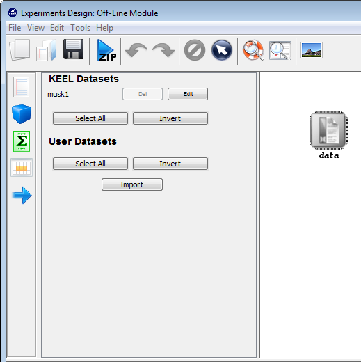

8 Appendix
In this section, we provide the unit test routines performed to the KEEL software:
- Scripts:
 72.4MB
- Results: 118.5MB
|
Copyright 2004-2018,
KEEL (Knowledge Extraction based on Evolutionary Learning)
About the Webmaster Team |

|