
Missing Values in Data Mining
- J. Luengo, S. García, F. Herrera, A Study on the Use of Imputation Methods for Experimentation with Radial Basis Function Network Classifiers Handling Missing Attribute Values: The good synergy between RBFs and EventCovering method. Neural Networks, 23(3) (2010) 406-418. doi:10.1016/j.neunet.2009.11.014

- J. Luengo, S. García, F. Herrera, On the choice of the best imputation methods for missing values considering three groups of classification methods. Knowledge and Information Systems 32:1 (2012) 77-108, doi:10.1007/s10115-011-0424-2 COMPLEMENTARY MATERIAL to the paper here: Software, data sets, results and methods description,.
- J. Luengo, José A. Sáez, F. Herrera, Missing data imputation for Fuzzy Rule Based Classification Systems. Soft Computing 16 (2012) 863–881 oi: 10.1007/s00500-011-0774-4.
The web is organized according to the following summary:
- Introduction to Missing Values Imputation in Data Mining
- Imputation Methods
- Technical description report
- On the suitability of imputation methods for different learning approaches
- Quantifying the effects of the imputation methods in the noise and information contained in the data set
- Data-sets partitions employed in the papers
- Complementary material of the papers
- WEB sites devoted to Missing Values
- Missing Values Bibliography
Introduction to Missing Values Imputation in Data Mining
Many existing, industrial and research data sets contain Missing Values. They are introduced due to various reasons, such as manual data entry procedures, equipment errors and incorrect measurements. Hence, it is usual to find missing data in most of the information sources used. The detection of incomplete data is easy in most cases, looking for Null values in a data set. However, this is not always true, since Missing Values (MVs) can appear with the form of outliers or even wrong data (i.e. out of boundaries).
Many existing, industrial and research data sets contain Missing Values. They are introduced due to various reasons, such as manual data entry procedures, equipment errors and incorrect measurements. Hence, it is usual to find missing data in most of the information sources used. The detection of incomplete data is easy in most cases, looking for Null values in a data set. However, this is not always true, since Missing Values (MVs) can appear with the form of outliers or even wrong data (i.e. out of boundaries).
Missing values make it difficult for analysts to perform data analysis. Three types of problems are usually associated with missing values (J. Barnard, X.L. Meng. Applications of multiple imputation in medical studies: From AIDS to NHANES. Stat. Methods Med. Res., 8 (1) (1999) 17-36, doi: 10.1191/096228099666230705 ![]() ):
):
- loss of efficiency;
- complications in handling and analyzing the data;
- bias resulting from differences between missing and complete data.
Farhangfar et al (A. Farhangfar, L. Kurgan, J. Dy. Impact of imputation of missing values on classification error for discrete data. Pattern Recognition 41 (2008) 3692-3705, doi: 10.1016/j.patcog.2008.05.019 ![]() ) summarize the three major approach to deal with MVs. The simplest way of dealing with missing values is to discard the examples that contain the missing values. However, this method is practical only when the data contain relatively small number of examples with missing values and when analysis of the complete examples will not lead to serious bias during the inference. Another approach is to convert the missing values into a new value (encode them into a new numerical value), but such simplistic method was shown to lead to serious inference problems. On the other hand, if a significant number of examples contain missing values for relatively small number of attributes, it may be beneficial to perform imputation (filling-in) of the missing values.
) summarize the three major approach to deal with MVs. The simplest way of dealing with missing values is to discard the examples that contain the missing values. However, this method is practical only when the data contain relatively small number of examples with missing values and when analysis of the complete examples will not lead to serious bias during the inference. Another approach is to convert the missing values into a new value (encode them into a new numerical value), but such simplistic method was shown to lead to serious inference problems. On the other hand, if a significant number of examples contain missing values for relatively small number of attributes, it may be beneficial to perform imputation (filling-in) of the missing values.
We will center our attention on the use of imputation methods. A fundamental advantage of this approach is that the missing data treatment is independent of the learning algorithm used. For this reason, the user can select the most appropriate method for each situation he faces. There is a wide family of imputation methods, from mean imputation to those which analyze the relationships between attributes.
In the other hand, it is important to categorize the mechanisms which lead to the introduction of MVs (R.J. Little and D.B. Rubin. Statistical analysis with Missing Data. John Wiley and Sons, New York, 1987). Such mechanism will determine which imputation method could be applied, if any. As Little and Rubin stated, there exist three different mechanism of missing data induction.
- Missing completely at random (MCAR), when the distribution of an example having a missing value for an attribute does not depend on either the observed data or the missing data.
- Missing at random (MAR), when the distribution of an example having a missing value for an attribute depends on the observed data, but does not depend on the missing data.
- Not missing at random (NMAR), when the distribution of an example having a missing value for an attribute depends on the missing values.
In case of the MCAR mode, the assumption is that the distributions of missing and complete data are the same, while for MAR mode they are different, and the missing data can be predicted by using the complete data (R.J. Little and D.B. Rubin. Statistical analysis with Missing Data. John Wiley and Sons, New York, 1987). These two mechanisms are assumed by the most imputation methods so far.
Imputation Methods
There exist many imputation methods published, but their use in the Data Mining field is limited. A very recent study only mention 4 big MVs studies in this field (A. Farhangfar, L. Kurgan, J. Dy. Impact of imputation of missing values on classification error for discrete data. Pattern Recognition 41 (2008) 3692-3705, doi: 10.1016/j.patcog.2008.05.019 ![]() ). Deeper searchs cand find some extra studies with less magnitude.
). Deeper searchs cand find some extra studies with less magnitude.
However, methods from other related fields can be adapted to be used as imputation methods. The imputation methods we have considered are briefly described next:
- Do Not Impute (DNI). As its name indicates, all the missing data remains unreplaced, so the networks must use their default MVs strategies. We want to verify whether imputation methods allow the Data Mining method to perform bet- ter than using the original data sets. As guideline, we find a previous study of imputation methods in (J.W. Grzymala-Busse, M. Hu. A Comparison of Several Approaches to Missing Attribute Values in Data Mining. In Rough Sets and Current Trends in Computing : Second In- ternational Conference (RSCTC 2000), Lecture Notes in Computer Science 2005, 2001, 378-385, ). However, no Machine Learning method is used after the imputation process.
- Case deletion or Ignore Missing(IM). Using this method, all instances with at least one MV are discarded from the data set.
- Global Most Common Attribute Value for Symbolic Attributes, and Global Average Value for Numerical Attributes (MC). (J.W. Grzymala-Busse, L.K. Goodwin. Handling Missing Attribute Values in preterm birth data sets. In Rough Sets, Fuzzy Sets, Data Mining, and Granular Computing (RSFDGrC 2005), Lecture Notes in Computer Science 3642, 2005, 342-351, ). This method is very simple: for nominal attributes, the MV is replaced with the most common attribute value, and numerical values are replaced with the average of all values of the corresponding attribute.
- Concept Most Common Attribute Value for Symbolic Attributes, and Concept Average Value for Numerical Attributes (CMC). (J.W. Grzymala-Busse, L.K. Goodwin. Handling Missing Attribute Values in preterm birth data sets. In Rough Sets, Fuzzy Sets, Data Mining, and Granular Computing (RSFDGrC 2005), Lecture Notes in Computer Science 3642, 2005, 342-351, ). As stated in MC, we replace the MV by the most repeated one if nominal or the mean value if numerical, but considering only the instances with same class as the reference instance.
- Imputation with K-Nearest Neighbour (KNNI). (G.E.A.P.A. Batista, M.C. Monard. An analysis of four missing data treatment methods for supervised learning. Applied Artificial Intelligence 17 (2003) 519-533, ). Using this instance-based algorithm, every time we found a MV in a current instance, we compute the k nearest neighbours and impute a value from them. For nominal values, the most common value among all neighbours is taken, and for numerical values we will use the average value. Indeed, we need to define a proximity measure between instances. We have chosen euclidean distance (it is a case of a Lp norm distance), which is usually used.
- Weighted imputation with K-Nearest Neighbour (WKNNI). (O. Troyanskaya, M. Cantor, G. Sherlock, P. Brown , T. Hastie, R. Tibshirani, D. Botstein, R.B. Altman. Missing value estimation methods for DNA microarrays. Bioinformatics 17 (2001) 520-525, ). The Weighted K-Nearest Neighbour method selects the instances with similar values (in terms of distance) to a considered one, so it can impute as KNNI does. However, the estimated value now takes into account the differ- ent distances to the neighbours, using a weighted mean or the most repeated value according to the distance.
- K-means Clustering Imputation (KMI). (D. Li, J. Deogun, W. Spaulding. Towards Missing Data Imputation: A Study of Fuzzy K-means Clustering Method. Rough Sets and Current Trends in Computing. Lecture Notes in Computer Science 3066, 2004 (2004) 573-579, ). Given a set of objects, the overall objective of clustering is to divide the data set into groups based on similarity of objects, and to minimize the intra-cluster dissimilarity. In K-means clustering, the intra-cluster dissimilarity is measured by the addi- tion of distances among the objects and the centroid of the cluster which they are assigned to. A cluster centroid represents the mean value of the objects in the cluster. Once the clusters have converged, the last process is to fill in all the non-reference attributes for each incomplete object based on the cluster information. Data objects that belong to the same cluster are taken as near- est neighbours of each other, and we apply a nearest neighbour algorithm to replace missing data, in a similar way than k-Nearest Neighbour Imputation.
- Imputation with Fuzzy K-means Clustering (FKMI). (E. Acuna, C. Rodriguez. The treatment of missing values and its effect in the classifier accuracy. In: W. Gaul, D. Banks, L. House, F.R. McMorris, P. Arabie (Eds.) Classification, Clustering and Data Mining Applications, Springer-Verlag Berlin-Heidelberg, 2004, 639-648, ). In fuzzy clustering, each data object xi has a membership function which describes the degree which this data object belongs to a certain cluster vk. In the process of updating membership functions and centroids, we only take into account only complete attributes. In this process, we cannot assign the data object to a concrete cluster represented by a cluster centroid (as done in the basic K-mean clustering algorithm), because each data object belongs to all K clusters with different membership degrees. We replace non-reference attributes for each incomplete data object xi based on the information about membership degrees and the values of cluster centroids.
- Support Vector Machines Imputation (SVMI). (H.A.B. Feng, G.C. Chen, C.D. Yin, B.B. Yang, Y.E. Chen. A SVM regression based approach to filling in missing values. Knowledge-Based Intelligent Information and Engineering Systems (KES05). Lecture Notes in Computer Science 3683, 2005 (2005) 581-587, ) is a SVM regression based algorithm to fill in missing data, i.e. set the decision attributes (output or classes) as the condition attributes (input attributes) and the con- dition attributes as the decision attributes, so we can use SVM regression to predict the missing condition attribute values. In order to do that, first we select the examples in which there are no missing attribute values. In the next step we set one of the condition attributes (input attribute), some of those values are missing, as the decision attribute (output attribute), and the decision attributes as the condition attributes by contraries. Finally, we use SVM regression to predict the decision attribute values.
- Event Covering (EC). (A.K.C. Wong and D.K.Y. Chiu. Synthesizing statistical knowledge from incomplete mixed- mode data. IEEE Transactions on Pattern Analysis and Machine Intelligence 9 (1987) 796-805 ). Based on the work of Wong et al., a mixed-mode probability model is approximated by a discrete one. First, they discretize the continuous components using a minimum loss of information criterion. Treating a mixed-mode feature n-tuple as a discrete-valued one, the authors propose a new statistical approach for synthesis of knowledge based on cluster analysis. As main advantage, this method does not require neither scale normalization nor ordering of discrete values. By synthesis of the data into statistical knowledge, they refer to the following processes: 1) synthesize and detect from data inherent patterns which indicate statistical interdependency; 2) group the given data into inherent clusters based on these detected interdependency; and 3) interpret the underlying patterns for each clusters identified. The method of synthesis is based on author's event{covering approach. With the developed inference method, we are able to estimate the MVs in the data.
- Regularized Expectation-Maximization (EM). (T. Schneider. Analysis of incomplete climate data: Estimation of Mean Values and covariance matrices and imputation of Missing values. Journal of Climate 14 (2001) 853-871, ). Missing values are imputed with a regularized expectation maximization (EM) algorithm. In an iteration of the EM algorithm, given estimates of the mean and of the covariance matrix are revised in three steps. First, for each record with missing values, the regression parameters of the variables with missing values on the variables with available values are computed from the estimates of the mean and of the covariance matrix. Second, the missing values in a record are filled in with their conditional expectation values given the available values and the estimates of the mean and of the covariance matrix, the conditional expectation values being the product of the available values and the estimated regression coe±cients. Third, the mean and the covariance matrix are re-estimated, the mean as the sample mean of the completed data set and the covariance matrix as the sum of the sample covariance matrix of the completed data set and an estimate of the conditional covariance matrix of the imputation error. The EM algorithm starts with initial estimates of the mean and of the covariance matrix and cycles through these steps until the imputed values and the estimates of the mean and of the covariance matrix stop changing appreciably from one iteration to the next.
- Singular Value Decomposition Imputation (SVDI). (O. Troyanskaya, M. Cantor, G. Sherlock, P. Brown , T. Hastie, R. Tibshirani, D. Botstein, R.B. Altman. Missing value estimation methods for DNA microarrays. Bioinformatics 17 (2001) 520-525, ). In this method, we employ singular value decomposition to obtain a set of mutually orthogonal expression patterns that can be linearly combined to approximate the values of all attributes in the data set. In order to do that, first we estimate the MVs with the EM algorithm, and then we compute the Singular Value Decomposition and obtain the eigenvalues. Now we can use the eigenvalues to apply a regression over the complete attributes of the instance, to obtain an estimation of the MV itself.
- Bayesian Principal Component Analysis (BPCA). (S. Oba, M. Sato, I. Takemasa, M. Monden, K. Matsubara and S. Ishii. A Bayesian missing value estimation method for gene expression profile data. Bioinformatics, 19 (2003) 2088-2096, doi: 10.1093/bioinformatics/btg287 ). This method is an estimation method for missing values, which is based on Bayesian principal component analysis. Although the methodology that a probabilistic model and latent variables are estimated simultaneously within the framework of Bayes inference is not new in principle, actual BPCA implementation that makes it possible to estimate arbitrary missing variables is new in terms of statistical methodology. The missing value estimation method based on BPCA consists of three elementary processes. They are (1) principal compo- nent (PC) regression, (2) Bayesian estimation, and (3) an expectationmaxi- mization (EM)-like repetitive algorithm.
- Local Least Squares Imputation (LLSI). (H.A. Kim, G.H. Golub, H. Park. Missing value estimation for DNA microarray gene expression data: Local least squares imputation. Bioinformatics, 21 (2) (2005) 187-198, doi: 10.1093/bioinformatics/bth499 ). With this method, a target instance that has missing values is represented as a linear combination of similar instances. Rather than using all available genes in the data, only similar genes based on a similarity measure are used the method has the "local" connotation. There are two steps in the LLSI. The first step is to select k genes by the L2-norm. The second step is regression and estimation, regardless of how the k genes are selected. A heuristic k parameter selection method is used by the authors.
Technical description report
This Section presents a collection of the complete technical description of the Missing Values methods listed in the previous section. We have maintained the same notation and formulation than the original reference papers where the imputation methos were originally presented.
Imputation of Missing Values. Method's Description. ![]()
Open source implementations of these methods can be found in KEEL Software
![]()
On the suitability of imputation methods for different learning approaches
The literature on imputation methods in data mining employs well-known machine learning methods for their studies, in which the authors show the convenience of imputing the MVs for the mentioned algorithms, particularly for classification. The vast majority of MVs studies in classification usually analyze and compare one imputation method against a few others under controlled amounts ofMVs and induce them artificially with known mechanisms and probability distributions (Acuna E, Rodriguez C (2004) Classification, clustering and data mining applications. Springer, Berlin, pp 639–648, Batista G., Monard M. (2003) An analysis of four missing data treatment methods for supervised learning. Appl Artif Intell 17(5):519–533, Farhangfar A., Kurgan L., Dy J. (2008) Impact of imputation of missing values on classification error for discrete data. Pattern Recognit 41(12):3692–3705, Hruschka E.R. Jr., Hruschka E.R., Ebecken N.F. (2007) Bayesian networks for imputation in classification problems. J Intell Inf Syst 29(3):231–252 )
In this context, more information needs to be given in order to establish the best imputation strategy for each classifier. It is reasonable to expect that similar classifiers will have similar response to the same imputation data. We will establish three groups of classifiers to categorize them, and we will examine the best imputation strategies for each group. The former groups are as follows:
- The first group consists of the rule induction learning category. This group refers to algorithms that infer rules using different strategies. Therefore,we can identify as belonging to this category those methods that produce a set of more or less interpretable rules. These rules include discrete and/or continuous features, which will be treated by each method depending on their definition and representation. This type of classificationmethods has been the most used in case of imperfect data (Qin B., Xia Y., Prabhakar S. (2011) Rule induction for uncertain data. Knowl Inf Syst, doi:10.1007/ s10115-010-0335-7, (in press)).
- The second group represents the approximate models. It includes artificial neural networks, support vector machines, and statistical learning. In this group, we include the methods that act like a black box. Therefore, those methods that do not produce an interpretable model fall under this category. Although the Naïve Bayes method is not a completely black box method, we have considered that this is the most appropriate category for it.
- The third and last group corresponds to the lazy learning category. This group includes methods that do not create any model, but use the training data to perform the classification directly. This process implies the presence of measures of similarity of some kind. Thus, the methods that use a similarity function to relate the inputs to the training set are considered as belonging to this category.
The complete relation of classifiers analyzed follows:
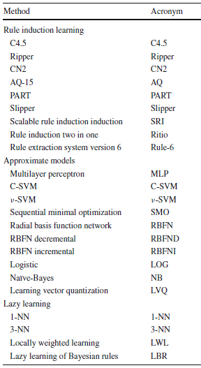
Classifiers considered for each category
By means of a large number of data sets (see next section), the best imputation strategy can be established for each classifier. We consider the use of the non-parametric pairwise statistical test formerly known as the Wilcoxon Signed Rank test to do so. Using this statistical test, each imputation method is compared against the others for each classifier. A final rank will establish the best imputation method for such classifier. The document with the final Wilcoxon's test results follows:
Tables with the Wilcoxon Signed Rank test results summarized for each classification method ![]()
The procedure followed in order to obtain the tables follows:
- We create a n x n table for each classification method. In each cell, the outcome of the Wilcoxon signed rank test is showed.
- In the aforementioned tables, if the p-value obtained by the Wilcoxon tests for the considered classification for a pair of imputation methods is higher than our a level, formerly 0.1, then we establish that there is a tie in the comparison (e.g. no significant difference was found), represented by a D in the cell.
- If the p-value obtained by the Wilcoxon tests is lower than our a level, formerly 0.1, then we establish that there is a win (represented by a W) or a loss (represented by a L) in the comparison. If the method presented in the row has better ranking than the method presented in the column in the Wilcoxon test then is a win, otherwise is a loss.
Then for each table we have attached three extra columns.
- The column "Ties+Wins" represents the amount of D and W present in the row. That is, the number of times that the imputation method performs better or equal than the rest for the classifier.
- The column "Wins" represents the amount of W present in the row. That is, the number of times that the imputation method performs better than the rest for the classifier.
- The column "RANKING" shows the average ranking derived from the two previous columns. The higher "Ties+Wins" has the method, the better. If there is a draw for "Ties+Wins", then the "Wins" are used in order to break the tie. Again, the higher "Wins" has the method, the better. If there also exists a tie in the "Wins", then an average ranking is established for all the tied methods mi to mj, given by:
$$RANKING = \frac{lRank(m_i,m_{i+1},...,m_j)+hRank(m_i,m_{i+1},...,m_j}{2}$$
where lRank() represents the lower ranking that all the methods can obtain (e.g. the last assigned ranking plus 1) and hRank() represents the highest possible rank for all the methods, that is
$$hRank(m_i,m_{i+1},...,m_j)=lRank(m_i,m_{i+1},...,m_j)+|{m_i,...m_j}|$$
Aggregating the best imputation method information obtained for each classifier using the aforementioned classifier categories, a final ranking of the best imputation strategy for each category can be stated. The following tables show the best imputation methods for each category and it can be seen that they differ from one category to another.
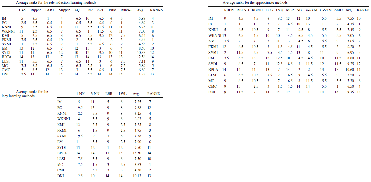
Imputation methods' ranking for each classifier category
From these tables, the best imputation method for each category are the following:
- FKMI, SVMI and EC methods for the rule induction learning algorithms.
- FKMI, SVMI and EC methods for the approximate models.
- MC, CMC and FKMI methods for the lazy learning models.
These results agree with the previous studies:
- The imputation methods that fill in the MVs outperform the case deletion (IM method) and the lack of imputation (DNI method).
- There is no universal imputation method that performs best for all classifiers.
From the results shown, the use of the FKMI and EC imputation methods is the best choice under general assumptions but showing little advantage with respect to the rest of imputation methods analyzed.
The particular analysis of the MVs treatment methods conditioned to the classification methods’ groups seems necessary. Thus, we can stress the recommended imputation algorithms to be used based on the classification method’s type, as in case of the FKMI imputation method for the rule induction learning group, the EC method for the approximate models and the MC method for the lazy learning models. We can confirm the positive effect of the imputation methods and the classifiers’ behavior and the presence of more suitable imputation methods for some particular classifier categories than others.
Quantifying the effects of the imputation methods in the noise and information contained in the data set
It is also interesting to relate the influence of the imputation methods to the performance obtained by the classification method based on the information contained in the data set. In order to study this influence and the benefits/drawbacks of using the different imputation methods, we have considered the use of two different measures. They are described as follows:
Wilson’s Noise Ratio: This measure proposed by Wilson (Wilson D. (1972) Asymptotic properties of nearest neighbor rules using edited data. IEEE Trans SystMan Cybern 2(3):408–421) observes the noise in the data set. For each instance of interest, the method looks for the K nearest neighbors (using the Euclidean distance) and uses the class labels of such neighbors in order to classify the considered instance. If the instance is not correctly classified, then the variable noise is increased by one unit. Therefore, the final noise ratio will be
$$Wilson's \ Noise = \frac{noise}{\# \ instances \ in\ the\ data\ set}$$
Mutual information (MI) is considered to be a good indicator of relevance between two random variables [12]. In our approach, we calculate the MI between each input attribute and the class attribute, obtaining a set of values, one for each input attribute MI($x_i$). In the next step, we compute the ratio between each one of these values, considering the imputation of the data set with one imputation method in respect of the not imputed data set. The average of these ratios will show us if the imputation of the data set produces a gain in information:
$$Avg. \ MI \ Ratio = \frac{\sum_{x_i \in X}{\frac{MI_{\alpha}(x_i)+1}{MI(x_i)+1}}}{|X|}$$
Averaging the rankings of Wilson's noise and Mutual Information for each imputation across all the data sets considered (see next section), we can establish the imputation method which introduces less noise and the imputation method which produces a greatest gain of information.
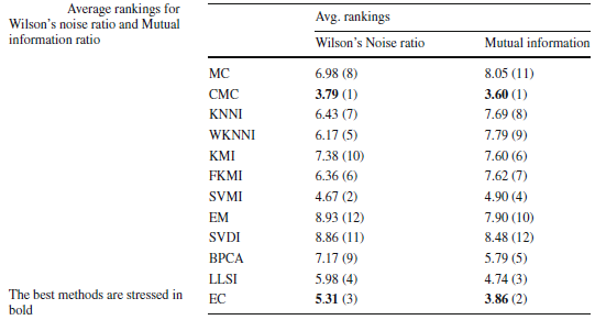
With the analysis performed, we have quantified the noise induced by the imputation methods and how the relationship between each input attribute and the class is maintained. We have shown that the CMC and EC methods show good behavior for these two measures, and they are two methods that provide good results for an important range of learning methods, as we have previously analyzed. In short, these two approaches introduce less noise and maintain the mutual information better.
Data-sets partitions employed in the papers
Below you can find all the Missing values data sets available. For each data set, it is shown its name and its number of instances, attributes, classes (number of possible values of the output variable) and the percentages of values with missing values and examples with missing values.
The table allows to download each data set in KEEL format (inside a ZIP file). Additionally, it is possible to obtain the data set from the KEEL Dataset Repository
![]()
| Data set | Acronym | #Examples | #Attributes | #Classes | %MVs (Values) | %MVs (Examples) | Download |
| Cleveland | CLE | 303 | 14 | 5 | 0,14 | 1,98 | |
| Wisconsin | WIS | 699 | 10 | 2 | 0,23 | 2,29 | |
| Credit | CRX | 689 | 16 | 2 | 0,61 | 5,37 | |
| Breast | BRE | 286 | 10 | 2 | 0,31 | 3,15 | |
| Autos | AUT | 205 | 26 | 6 | 1,11 | 22,44 | |
| Primary tumor | PRT | 339 | 18 | 21 | 3,69 | 61,06 | |
| Dermatology | DER | 365 | 35 | 6 | 0,06 | 2,19 | |
| House-votes-84 | HOV | 434 | 17 | 2 | 5,3 | 46,54 | |
| Water-treatment | WAT | 526 | 39 | 13 | 2,84 | 27,76 | |
| Sponge | SPO | 76 | 46 | 12 | 0,63 | 28,95 | |
| Bands | BAN | 540 | 40 | 2 | 4,63 | 48,7 | |
| Horse-colic | HOC | 368 | 24 | 2 | 21,82 | 98,1 | |
| Audiology | AUD | 226 | 71 | 24 | 1,98 | 98,23 | |
| Lung-cancer | LUN | 32 | 57 | 3 | 0,27 | 15,63 | |
| Hepatitis | HEP | 155 | 20 | 2 | 5,39 | 48,39 | |
| Mushroom | MUS | 8124 | 23 | 2 | 1,33 | 30,53 | |
| Post-operative | POS | 90 | 9 | 3 | 0,37 | 3,33 | |
| Echocardiogram | ECH | 132 | 12 | 4 | 4,73 | 34,09 | |
| Soybean | SOY | 307 | 36 | 19 | 6,44 | 13,36 | |
| Mammographic | MAM | 961 | 6 | 2 | 2,81 | 13,63 | |
| Ozone | OZO | 2534 | 73 | 2 | 8,07 | 27,11 |
Next, it provides a set of classification data set with missing values induced. They are modified version from those that can be found in the Standard classification data sets category of the KEEL repository, where a 10% of values have been randomly removed (only training partitions present missing values. Test partitions remains unchanged).
For each data set, it is shown its name and its number of instances, attributes (Real/Integer/Nominal valued), classes (number of possible values of the output variable) and the percentages of values with missing values and examples with missing values.
The table allows to download 10-folds cross validation partitions of each data set in KEEL format (inside a ZIP file)
| Name | #Attributes (R/I/N) | #Examples | #Classes | %MVs (Values) | %MVs (Examples) | Download |
|---|---|---|---|---|---|---|
| Iris+MV | 4 (4/0/0) | 150 | 3 | 10.00 % | 32.67 % | |
| Pima+MV | 8 (8/0/0) | 768 | 2 | 10.00 % | 50.65 % | |
| Wine+MV | 13 (13/0/0) | 178 | 3 | 10.00 % | 70.22 % | |
| Australian+MV | 14 (3/5/6) | 690 | 2 | 10.00 % | 70.58 % | |
| Newthyroid+MV | 5 (4/1/0) | 215 | 3 | 10.00 % | 35.35 % | |
| Ecoli+MV | 7 (7/0/0) | 3336 | 8 | 10.00 % | 48.21 % | |
| Satimage+MV | 36 (0/36/0) | 6435 | 7 | 10.00 % | 87.80 % | |
| German+MV | 20 (0/7/13) | 1000 | 2 | 10.00 % | 80.00 % | |
| Magic+MV | 10 (10/0/0) | 1902 | 2 | 10.00 % | 58.20 % | |
| Shuttle+MV | 9 (0/9/0) | 2175 | 7 | 10.00 % | 55.95 % |
Also, you can download all datasets by clicking ZIP file ![]()
Complementary material of the papers
This section gathers the particular imputed data sets and the results obtained for each paper.
A Study on the Use of Imputation Methods for Experimentation with Radial Basis Function Network Classifiers Handling Missing Attribute Values: The good synergy between RBFs and EventCovering method
 |
J. Luengo, S. García, F. Herrera, A Study on the Use of Imputation Methods for Experimentation with Radial Basis Function Network Classifiers Handling Missing Attribute Values: The good synergy between RBFs and EventCovering method. Neural Networks 23 406-418, doi:10.1016/j.neunet.2009.11.014. |
Abstract:
The presence of Missing Values in a data set can affect the performance of a classifier constructed using that data set as a training sample. Several methods have been proposed to treat missing data and the one used more frequently is the imputation of the Missing Values of an instance.
In this paper, we analyze the improvement of performance on Radial Basis Function Networks by means of the use of several imputation methods in the classification task with missing values. The study has been conducted using data sets with real Missing Values, and data sets with artificial Missing Values. The results obtained show that EventCovering offers a very good synergy with Radial Basis Function Networks. It allows us to overcome the negative impact of the presence of Missing Values to a certain degree.
Summary:
- Introduction
- Preliminaries: Missing values, imputation methods and their use in Neural Networks
- Experimental study: Imputation methods
- Concluding remarks
Experimental study:
Algorithms analyzed: RBFN, RBNFD, RBNFI (Neural Networks) IM, EC, KNNI, WKNNI, KMI, FKMI, SVMI, EM, SVDI, BPCA, MC, CMC, DNI (Imputation Methods)
Data sets used: ZIP file ![]()
Missing values: [10fcv] Australian+MV, Autos, Bands, Breast, Cleveland, Crx, Ecoli+MV, German+MV, Hepatitis, Horse-colic, House-Votes-84, Iris+MV, Magic+MV, Mammographic, Mushroom, New-thyroid+MV, Pima+MV, Post-operative, Satimage+MV, Shuttle+MV, Wine+MV, Wisconsin
Results obtained: ZIP file ![]()
| XLS file |
CSV file |
RBFN results |
| XLS file |
CSV file |
RBFND results |
| XLS file |
CSV file |
RBFND results |
On the choice of the best imputation methods for missing values considering three groups of classification methods
 |
J. Luengo, S. García, F. Herrera, On the choice of the best imputation methods for missing values considering three groups of classification methods. Knowledge and Information Systems, in press (2011). doi:10.1007/s10115-011-0424-2 |
Abstract:
In real-life data, information is frequently lost in data mining, caused by the presence of missing values in attributes. Several schemes have been studied to overcome the drawbacks produced by missing values in data mining tasks; one of the most well known is based on preprocessing, formerly known as imputation. In this work, we focus on a classification task with twenty-three classification methods and fourteen different imputation approaches to missing values treatment that are presented and analyzed. The analysis involves a group-based approach, in which we distinguish between three different categories of classificationmethods. Each category behaves differently, and the evidence obtained shows that the use of determined missing values imputation methods could improve the accuracy obtained for these methods. In this study, the convenience of using imputation methods for preprocessing data sets with missing values is stated. The analysis suggests that the use of particular imputation methods conditioned to the groups is required.
Summary:
- Introduction
- Imputation background
- Experimental framework
- Experimental results
- Influence of the imputation on the instances and individual features
- Lessons learned
Experimental study:
Algorithms analyzed: IM, EC, KNNI, WKNNI, KMI, FKMI, SVMI, EM, SVDI, BPCA, LLSI, MC, CMC, DNI (Imputation Methods). RBFN, RBFND, RBFNI, C4.5, 1-NN, LOG, LVQ, MLP, NB, nu-SVM, C-SVM, Ripper, PART, Slipper, 3-NN, AQ, CN2, SMO, LBR, LWL, SRI, Ritio, Rule-6 (Classification Methods).
Data sets used: ZIP file ![]()
Missing values: [10fcv] Cleveland, Wisconsin, Credit, Breast, Autos, Primary tumor, Dermatology, House-votes-84, Water-treatment, Sponge, Bands, Horse-colic, Audiology, Lung-cancer, Hepatitis, Mushroom, Post-operative, Echocardiogram, Soybean, Mammographic and Ozone
Results obtained: ZIP file ![]()
|
XLS file |
CSV file |
C4.5 results |
|
XLS file |
CSV file |
Ripper |
|
XLS file |
CSV file |
CN2 results |
|
XLS file |
CSV file |
AQ-15 |
|
XLS file |
CSV file |
PART |
|
XLS file |
CSV file |
Slipper |
|
XLS file |
CSV file |
SRI results |
|
XLS file |
CSV file |
Ritio |
|
XLS file |
CSV file |
Rule-6 |
|
XLS file |
CSV file |
MLP |
|
XLS file |
CSV file |
C-SVM |
|
XLS file |
CSV file |
nu-SVM |
|
XLS file |
CSV file |
SMO |
|
XLS file |
CSV file |
RBFN |
|
XLS file |
CSV file |
RBFND |
|
XLS file |
CSV file |
RBFNI |
|
XLS file |
CSV file |
LOG |
|
XLS file |
CSV file |
NB results |
|
XLS file |
CSV file |
LVQ |
|
XLS file |
CSV file |
1-NN |
|
XLS file |
CSV file |
3-NN |
|
XLS file |
CSV file |
LWL |
|
XLS file |
CSV file |
LBR |
WEB sites devoted to Missing Values
- A complete Webpage devoted to MVs analysis and study metodology.
- Schafer's Multiple Imputation Webpage with Windows binaries.
- David C. Howell's Webpage devoted to the treatment of Missing Data with some examples.
- Regularized Expectation-Maximization Algorithm homepage with MATLAB code.
- BPCA homepage with MATLAB and Java code.
- LLSI homepage with MATLAB source code.
Bibliography compilation about the Missing Values in Data Mining
We have performed a bibliography compilation of journal papers on Missing Values in Data Mining. It is maintained by J. Luengo.
If you would like to include or correct any of the references on this page, please contact the maintainer in his e-mail address: julianlm@decsai.ugr.es